Guide to Mastering Electronics: Radio and television

Radio transmission and reception was perhaps one of the earliest applications of electronics, and is--so far--the application that has made the greatest impact on society. Oddly, we can use radio, predict its properties and design circuits that work very efficiently, but we know little about the real nature of radio. Ask an electronics engineer what radio is, and the answer will be a confident, 'Electromagnetic waves.' Ask a physicist what electromagnetic waves are, and he will begin to hedge, or he will tell you that really we don't know. We do know that electromagnetic radiation is a form of energy, and that it behaves as if it is propagated as waves. The model becomes more of a model and less like reality when we discover that radio travels through a vacuum. How can there be waves in a vacuum? Perhaps in the future, theoretical physics will give us an answer. In the meantime, we use radio, describe it mathematically, and design and use electronic circuits that function happily despite our underlying ignorance.

Possibly the hardest concept to grasp in radio is the way in which circuits can be made that broadcast radio waves into their surroundings.

We begin with the LC tuned circuit, given in Figure 10.20. You will remember how the circuit, when oscillating, stored all the available energy, first in the capacitor and then in the magnetic field associated with the inductor, reversing the situation with each swing of oscillation.

Consider the way in which energy is stored in the capacitor ( Section 3) it is in the form of an electric field, whatever that may be! All capacitors that we use in electronic circuits develop an electric field between two parallel and very closely spaced plates. Moving the plates apart has two effects. First, it decreases the capacitance (the principle of variable capacitors); and second it makes the electric field occupy a larger volume of space. We could make a capacitor with two plates a meter apart, which would give a tiny value of capacitance unless the plates were very large indeed.

Operating this cumbersome arrangement in an LC oscillator circuit would yield an unexpected result, for not all the energy put in to the circuit could be accounted for by waste heat emitted by the coil windings, etc. Some of the energy has escaped--leaked away, if you like--from the area between the plates (which are rather a long way apart). This escaped energy is, of course, electromagnetic or 'radio' energy, and has been broad cast away from the circuit. In order to make a radio transmitter, we need a circuit that will give the maximum possible 'leakage' of energy from the LC oscillator.

As you might expect from the hypothetical experiment outlined above, what is needed is a capacitor with an enormous gap between the plates, and designed in such a way that the largest possible amount of radio is 'leaked'. We can, in fact, use the largest possible plate for one of the plates of the capacitor-we can use the earth! The other 'plate' has to be rather smaller, and it is convenient to use a single, long wire; this has the advantage that it can be made an excellent 'leaker' of radio energy. The earth and wire as a capacitor is shown in Fig. 1. The picture is a familiar one, that of a radio aerial.

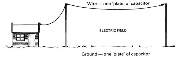
FIG. 1 an aerial --- Wire- one 'plate' of capacitor --- Ground- one 'plate' of capacitor.

It also turns out that there is an optimum length for the aerial wire, if the 'leakage', which I shall now call 'broadcast energy', is to be maximized.

Conveniently, it is when the aerial is half, or one-quarter, of the wave length. The term 'wavelength' refers to the physical distance between complete cycles of the broadcast wave. Radio waves travel at the speed of light, which is about 300 000 km per second. If the radio waves were produced at the highly unlikely rate of one a second, the wavelength would be 300,000 km. Two a second, and the wavelength would be 150000 km, still a little on the long side for a convenient aerial to be one quarter of the wavelength!

Radio is broadcast on much higher frequencies than this, but the formula for working out the wavelength is the same: A=~ f (where A is the Greek letter 'lambda', which is conventionally used to represent wavelength). At a radio frequency of 10 MHz, the wavelength would be A= 300000000 meters 10000000 A= 30m A convenient quarter-wavelength aerial would be 7.5 m, not too bad, but unsuitable for portable equipment. For portable radio transmitters, we can exchange convenience for efficiency, and use a 1/8 wavelength or a 1 /16 wavelength aerial.

The length of the aerial will affect the capacitance (refer to Fig. 1 and you will see why this happens) and this will affect the frequency of oscillation. For a transmitter circuit to work properly, the LC circuit must be 'tuned' to the transmission frequency, and the aerial must be the correct length. Radio frequencies between 30kHz and 20 GHz or so are used. Fig. 2 overleaf illustrates the different frequency 'bands' and the names given them.

1. RADIO TRANSMITIERS

We can now look at a practical transmitter circuit, operating in the high frequency band at 27 MHz. The choice of frequency is not arbitrary, for this is the model radio control frequency, and in the UK and many other countries it is legal to operate a low power transmitter at this frequency without any form of license. Many readers can therefore build and operate this circuit-provided it is properly tuned-without breaking the law.

In order to ensure that they are operating on a legal frequency, model control transmitters have to be crystal controlled, i.e. the frequency of oscillation must be controlled by a quartz crystal oscillator, to ensure accuracy and stability. A frequency close to the middle of the model control band is 27.095 MHz, and crystals at this frequency are readily available from good electronic component or model shops.

The crystal-controlled oscillator circuit in Figure 10.24 is a good starting-point. This oscillator provides the necessary radio frequency sinewave output, which is then amplified by a simple transistor amplifier.

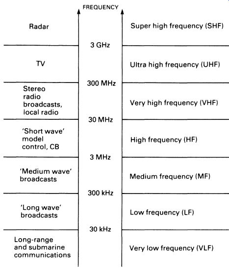
FIG. 2 the radio spectrum

Note the use of a tuned circuit for the transistor amplifier, something which is fairly common in radio circuits. The use of a tuned collector load improves the efficiency, for the impedance of the load is highest at the 'wanted' frequency, giving the best output and optimum bias. In this case the frequency of the resonant circuit is about 27.1 MHz.

The specification of inductors is always problematic, because there are many different ways of making, say, a 10 mH inductance, and not all are suitable for all applications. In practical circuits it is usual to give constructional details of any 'purpose-made' inductors, to ensure that the right design is used for the circuit. Fortunately for us, the amounts of inductance required in high frequency radio circuits are generally quite small, and suitable inductors are easily made with a few turns of enamel insulated wire over a small ferrite core (or no core, in which case the inductor is called 'air-cored'). To give a reasonable range with a typical model control receiver, our transmitter needs an output of 200-500 mW. A third, power stage, is used to give the high output current needed.

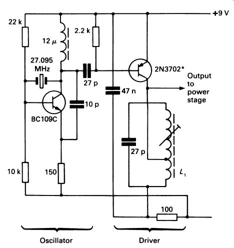
FIG. 3 a crystal-controlled oscillator circuit, followed by a tuned amplifier stage; this practical circuit can form the basis of a transmitter L, details 6'14 plus 3'14 turns of 24 s.w.g. enamel-insulated wire, wound on a '14 inch former with dust core (adjustable).

*For later projects in this guide, the 2N3702 emitter is disconnected from the positive supply. It is worth making the emitter accessible!

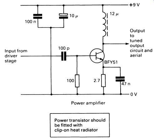
FIG. 4 the output stage of a small transmitter; this can be driven directly by the circuit in Fig. 3.

The power stage is very similar to the preceding stage, using a very simple transistor amplifier. However, a larger, high-power transistor is needed, and the collector load (and thus the bias resistor) are much smaller in value to provide the required current. The circuit is given in Fig. 4.

Notice the resistor values associated with the power stage, and notice also the small capacitor (100 pF) used for coupling the stage to the one preceding it: the high frequency means that a small capacitor is able to pass sufficient current.

The last part of the circuit, following the power stage, is the output tuning circuit. There are various forms, but it is usual to have two tuned circuits-both LC circuits--to improve efficiency. The circuit shown in Fig. 5 is typical.

There are a number of noteworthy points about this circuit. First, the inductors are generally air-cored (again, for efficiency) but may be wound on ferrite cores to increase the inductance if the transmitter has to be small. Second, the capacitors are variable, so that the circuit can be tuned accurately-the LC circuits have to be accurately 'peaked' (i.e. tuned to the exact frequency) for the transmitter to work properly. The same is true of any other tuned circuits, such as the collector load of the stage driving the power stage.

The capacitor that couples the aerial itself to the circuit is there for safety reasons, and does not play any part in the circuit's functioning. If the aerial is accidentally shorted to the transmitter casing (which is earthed to the 0 V power line) this would short-circuit the output transistor and could damage the driver transistor; but the 10 nF capacitor prevents this.

In practice, the circuit can be built on a printed board, and layout is uncritical. Matrix board is not suitable, since the strips of copper act as unwanted capacitors-at high frequencies a few picofarads can be import ant. The coils (in this design) are intended to be mounted facing the same way (i.e. with the same axis).

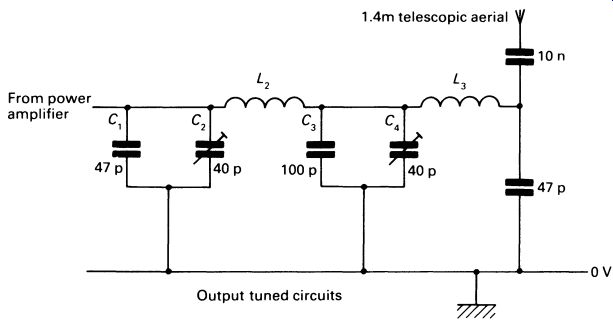
FIG. 5 output tuned circuits for a 27 MHz transmitter; this circuit can be driven directly by the output amplifier in Fig. 4 --------- L, L3 details each 12 turns of 18 s.w.g. wire, air core about 8 mm diameter. Wind so that the turns are touching; the coils can conveniently be wound round a pencil.

The circuit shown in Figures 4 and 5 is entirely practical, and can be made as a construction project. The crystal must be suitable for operating on the model control band, between 26.995 and 27.245 MHz in the UK. The transmitter can be built, but we need some kind of detector to check that it is working, and to allow us to tune the LC circuits. A suitable detector is shown in Fig. 6. This is very simple, and will react to the 27 MHz radio frequency when held a few centimeters from the transmitter aerial.

The radio signal induces a small current in the wire, and this flows through the meter. Without the diode, an alternating current would flow, which would not perceptibly affect the meter-the sluggish needle is unable to swing to and fro 27 million times a second! The diode rectifies the signal, and makes the current flow through the meter unidirectional.

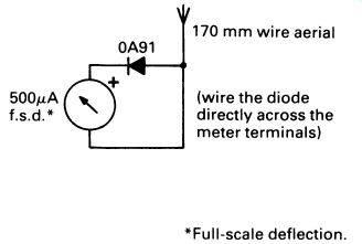
FIG. 6 an RF detector suitable for use with a low-power 27 MHz transmitter ----------- 170 mm wire aerial (wire the diode directly across the meter terminals). Full-scale deflection.

The meter can measure the current, and responds to the radio signal. Such a device is referred to as a detector, or RF meter (radio frequency meter). The diode specified is germanium, not silicon. Thermal effects and leakage are unimportant in this application, but forward voltage drop is-and the germanium diode is better than silicon in this respect (germanium semi conductors still have their place). The RF meter can be used to tune the transmitter. Connect the power supply to the transmitter, and bring the RF meter close up to the fully extended aerial. Adjust the core of L1 with a plastic screwdriver (not a metal one, which would affect the inductance). At one point, the meter will show a small deflection. Adjust the core for maximum deflection of the meter. Now adjust the output capacitors to improve the deflection.

You may need to move the RF meter further away from the aerial, but keep on adjusting Lt. C2 and C4 until no further improvement can be obtained. This is the way to ensure that all the tuned circuits are set as accurately as possible to 27.095 MHz.

The final adjustment should be made with the transmitter in its metal case, held in the hand. The reason is that the connection to earth is made through the operator, who will be holding the transmitter and will have his feet touching the ground.

2. MODULATION AND DEMODULATION

Although this transmitter can send out quite a powerful signal, the signal itself carries no information. The RF meter can detect the presence or absence of the signal, but if the radio waves are to carry useful information, such as speech or control signals, the system needs additions.

There are two common methods of adding information to the radio signal, which is called the carrier. Each involves changing the carrier slightly, and both systems are in common use. The first, and most obvious, is amplitude modulation (AM). Amplitude modulation involves nothing more complicated than changing the power, or amplitude, of the carrier in sympathy with the modulating signal. This is clearly illustrated in Fig. 7, which shows the carrier being modulated with an audio-frequency sinewave.

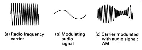
FIG. 7 amplitude modulation ------ • (a) Radio frequency carrier (b) Modulating audio signal (c) Carrier modulated with audio signal: AM

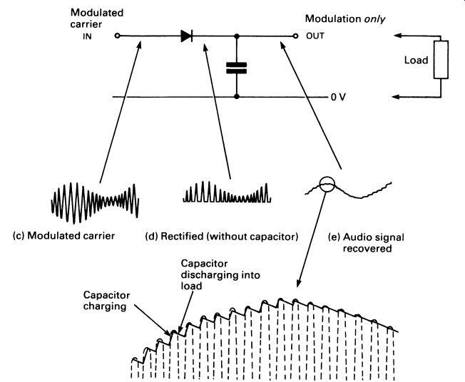
FIG. 8 detector circuit designed to recover an audio waveform from an AM radio signal ----------- (c) Modulated carrier (d) Rectified (without capacitor) (e) Audio signal recovered

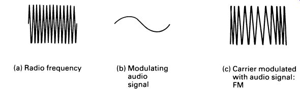
Fig 9 frequency modulation -------- • (a) Radio frequency (b) Modulating audio signal (c) Carrier modulated with audio signal: FM

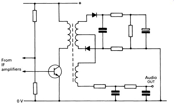
FIG. 10 a ratio detector circuit used for recovering the audio signal from an FM transmission

AM has the additional advantage that it is easy to recover, or detect at the receiver. Assuming that the signal received by the receiver is roughly the same as that shown in Fig. 7c, we cannot simply feed the output into a speaker. The output is, at audio frequencies, symmetrical so that any increase in positive signal is exactly balanced by a similar increase in negative signal and the result is zero.

Fortunately, the audio signal can be extracted simply by rectifying the receiver's output, to make it asymmetrical. The carrier is then removed with a small capacitor. The circuit is shown in Fig. 8, along with the waveforms associated with it. Comparison with Fig. 7 shows how the modulating waveform is recovered more or less unchanged.

The second method is known as frequency modulation (FM). Instead of changing the amplitude of the carrier in sympathy with the modulating waveform, the frequency is shifted a little higher or a little lower. The amount of frequency shift is very small. Frequency modulation of a carrier is illustrated in Fig. 9; compare it with the same diagram for amplitude modulation, Fig. 7.

Detection of the FM signal is much more complicated than detection of AM signals. Various circuits have been developed, and up to the beginning of the 'integrated-circuit era' a circuit known as a ratio detector was most commonly used to recover the modulating signal. The circuit is given in Fig. 10. The functioning of this circuit is quite complicated, and it is now little used.

Nowadays a circuit called phase-locked loop is often used. A system diagram is shown in Fig. 11. The circuit operates as follows. The frequency-modulated signal from the receiver is fed into one input of the phase detector. The other input of the phase detector is connected to the output of a voltage-controlled oscillator (VCO), working at the same frequency as the carrier. The phase detector compares the phases of the two signals--see Fig. 12--and, if the two signals are out of phase, produces a positive or negative output according to the direction of phase error.

The output is fed to the VCO, which changes frequency in such a way as to move its output signal back into phase with the incoming frequency modulated carrier. The VCO therefore 'tracks' the frequency changes of the carrier, continuously altering its own frequency to correspond with the incoming frequency modulation. The VCO 'locks' on to the carrier, through a feedback loop (hence 'phase-locked loop'). Now look at the control voltage applied to the VCO by the phase detector. A few moments' thought will show that this control voltage accurately reflects the changes in frequency of the incoming signal--it has to, in order to make the VCO change frequency to track the modulation. The control voltage therefore reproduces very accurately the modulating signal, and is simply amplified to provide an audio output.

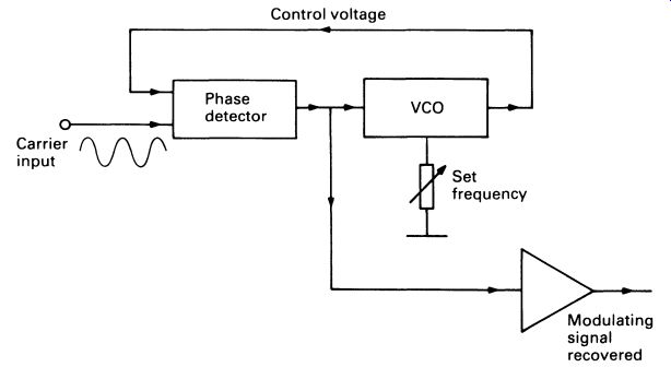
FIG. 11 system diagram for the phase-locked loop system of detecting a frequency-modulated signal

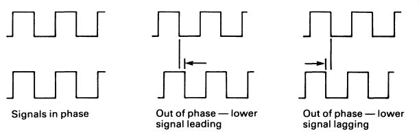
FIG. 12 signals in and out of phase.

Another, very important, advantage of the phase-locked loop is that it not only tracks the modulation but will, within a certain range, track overall changes in frequency of the carrier, or will compensate automatic ally for any 'drift' in its own operating parameters. This feature enables the detector to lock on to a signal when the receiver is tuned sufficiently nearly to the transmitter frequency. You will notice this feature working in almost all modern FM radio receivers.

Phase-locked loop integrated circuits specifically designed for radio receivers will usually incorporate other 'convenience' features. These include an output to operate an indicator (usually a LED) when the circuit is locked on to a signal, a means of turning off the feedback to unlock the circuit, and a means of changing the 'capture range' of the circuit (i.e. the amount of deviation from the selected frequency before the circuit unlocks). It is obvious that the phase-locked loop is actually a rather complicated circuit. Its internal design is certainly complex, but this is unimportant in the context of ICs. The IC is treated as a single component by manufacturers of radios, and as a 14--pin DIL pack (typical packaging for this component) it simplifies and cheapens assembly of an FM radio receiver.

To return to the practical transmitter circuit of Figures 3-5, the output can be amplitude-modulated by varying the gain of the driver stage with an applied signal. A simple way of doing this is to remove the base connection of the driver transistor from the positive supply rail and connect it to the output of an amplifier or transistor switch that can swing between 0V and the positive supply voltage. The output of the transmitter will vary in more or less linear fashion with the voltage. There are, of course, many different circuits for modulating a transmitter, all achieving the same result.

If the demonstration transmitter has been constructed, a modulator designed for model control can be added. Details are given in Section 22, since the pulse-width modulation system used involves digital systems. In the UK at least, it is illegal to add an audio modulator to this transmitter.

Fig. 13 illustrates the connection for the modulator-refer also to Fig. 3.

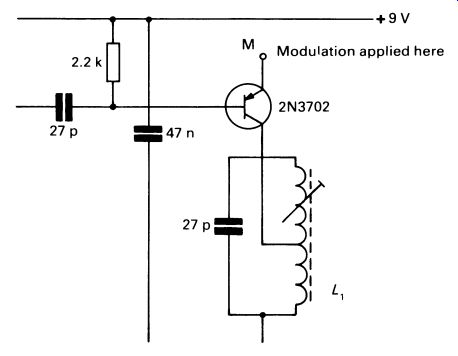
FIG. 13 modification to the transmitter circuit to enable modulation to be applied

Frequency-modulation techniques are beyond the scope of this guide, but a simple FM modulator uses a varicap diode, in parallel with the oscillator crystal, to obtain small changes in transmission frequency according to an applied modulating voltage.

3. RADIO RECEIVERS

The simplest radio receiver consists of just a tuned circuit, a diode, a capacitor, a pair of headphones, and as much aerial wire as possible! This is the 'crystal set' of the 1920s, and is shown in Fig. 14.

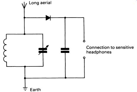
FIG. 14 a 'crystal set'

The electric field from the transmitter induces a tiny current in the aerial wire-which needs to be a few tens of meters long-and the LC resonant circuit selects the required frequency. It does this because the LC circuit has low impedance at frequencies other than the resonant frequency, and this 'shorts out' unwanted radio transmissions. At the resonant frequency the LC circuit has a high impedance, so the trans mission at the selected frequency appears across the circuit as a small radio frequency alternating voltage.

This is rectified by the diode to recover the audio signal, using a diode with a low forward voltage drop (germanium). The capacitor removes the RF component--Fig. 8-and a pair of sensitive high-impedance head phones produce a Gust) audible output.

The output can, of course, be amplified. However, results from this circuit are still unsatisfactory, chiefly because the tuning cannot separate one radio station from the next. Often, several stations will be received together.

There is a need to make the receiver more selective. As we saw earlier, when discussing transmitters, the use of a tuned LC circuit as a transistor amplifier's collector load-instead of a resistor--makes the circuit selective, amplifying the wanted frequency much more than other frequencies. If, therefore, a tuned transistor amplifier of this type follows the tuned aerial circuit, selectivity is enormously improved. The sensitivity of the receiver is also better, as the radio frequency signal is amplified before it reaches the detector diode. A receiver incorporating a single tuned RF amplifier is shown in Fig. 15.

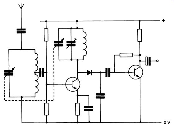
FIG. 15 TRF receiver: only moderately efficient

FIG. 16 circuit of a modern IC TRF receiver; this provides a low-level output suitable for feeding to an audio amplifier-this is a practical circuit and will work well with the amplifier designs of Figures 13.9 and 13.13

Receivers of this type can be made to work quite efficiently, and are very simple to construct. There is, in fact, an integrated circuit version of this tuned radio frequency (TRF) receiver, the ZN414. The ZN414 makes an ideal construction project as it is by far the simplest radio receiver to build. Unfortunately, it will not operate at frequencies higher than 3 MHz, so cannot be used with the model control transmitter. It can, however, be used very effectively with the amplifiers illustrated in Figure 13.9 and 13.3 and will connect directly to them. The circuit for the ZN414 radio is shown in Fig. 16. The two forward-biased diodes appear to short-circuit the power supply to the ZN414, but this IC requires only a 1.5 V supply, and the combined forward voltage drop of the diodes (0.7 V + 0.7 V = 1.4 V) produces a reference voltage that is near enough right. The circuit takes only 300-500 uA from the supply! There is no external aerial. With the sensitivity of the receiver vastly increased compared with the simple crystal set, the inductor itself can pick up a sufficiently large signal to work the receiver. A large ferrite core a few centimeters long is used for the aerial, with the coils of the inductor of the tuned aerial circuit wound on it. The whole assembly is called a ferrite rod aerial. The aerial is quite directional and can be used to tune out unwanted signals.

Although capable of a respectable performance, the TRF has definite limitations and the ZN414 may represent a development approaching the ultimate for this type of design.

A much better bet from the point of view of selectivity in particular is a receiver consisting of a number of tuned amplifier stages. It turns out that this is difficult to build, and even if built gives a poor audio quality. If an audio frequency signal is used to modulate a radio frequency carrier, the result will not be a signal at one frequency alone, but a signal that has components at a whole range of frequencies. The lowest will be the carrier frequency minus the highest audio frequency and the highest will be the carrier frequency plus the highest audio frequency. A medium wave radio station transmitting at 500kHz, with an audio signal between 40 and 9000Hz, would therefore actually be broadcasting on frequencies between 500- 9 =491kHz and 500 + 9 =509kHz. And the radio receiver would need to respond to all frequencies between these two figures equally, and ideally not respond at all to frequencies above 509kHz or below 491 kHz.

This is not possible to attain using a series of tuned circuits, for the combined effect is too selective at the chosen frequency.

Much more serious deficiencies come to light when we try to tune the receiver. With several stages, each with its own tuned circuit, we have to contrive a means of tuning every LC circuit simultaneously when changing frequency (station). Such a design would be very cumbersome, though a few were made in the 1930s.

There is a solution, one that is employed by all commercially made radio receivers. The design is called the superheterodyne (superhet) receiver, and a system diagram is given in Fig. 17.

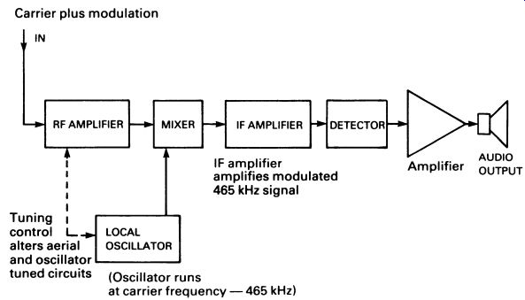
FIG. 17 system diagram for a superhet radio receiver.

The incoming signal from the radio frequency amplifier (the RF amplifier may be missing in very simple receivers) is mixed with a signal from an oscillator, known as the local oscillator. The oscillator is tuned to a slightly lower frequency than the selected radio frequency. In just the same way that the transmitter produced sum and difference frequencies above and below the carrier frequency, so the mixer produces an output that is the difference between the frequencies of the received radio signal and the output of the local oscillator. The oscillator is designed, in most AM receivers, to run precisely 465kHz below that of the received carrier. A ganged (double) variable capacitor is used to alter the tuning of the aerial circuit and the oscillator simultaneously, always keeping them 465 kHz apart. The output of the mixer is therefore always a 'carrier' at 465kHz, and this carrier is still modulated with the original audio signal.

Now it is possible to use two or three tuned amplifier stages if necessary.

The lower frequency makes design much easier, and the tuning of the stages can be arranged to give a selectivity response close to the ideal. Once the signal has been amplified sufficiently, a detector diode (or, for FM, a suitable discriminator circuit) can follow, with audio amplification last in the line.

The frequency resulting from the carrier and local oscillator inputs to the mixer is called the intermediate frequency (IF), and the stages that follow are called intermediate frequency amplifiers. They invariably have tuned collector loads: tuned, of course, to the intermediate frequency.

The intermediate frequency need not be 465kHz. In model control receivers it is usually 455kHz, and in VHF radio receivers it is 10.7 MHz.

The range of intermediate frequencies used is limited, not for any technical reasons but for the purely practical reason that manufacturers produce IF tuned transformers, known as intermediate frequency transformers (IFTs) that are preset to the intermediate frequency, and it is convenient to make just a few types. IF amplifier stages invariably use transformer coupling, for the tuned collector load simply needs a secondary winding to make it into a coupling transformer as well, which saves components and makes for an efficient circuit. A transformer-coupled amplifier stage was shown in Figure 10.11.

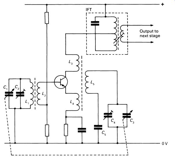
FIG. 18 mixer/oscillator stage, with a tuned collector load

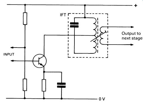
FIG. 19 a typical/ F amplifier stage

Receivers built with discrete components generally combined the local oscillator and mixer into a single transistor stage by means of a circuit like the one illustrated in Fig. 18. The inductor of the tuned circuit L 1 C1 +C2 is wound on the ferrite rod aerial, along with a coupling winding L 2 which works as a transformer and provides a signal current for the transistor. The transistor, as well as working as an RF amplifier, acts as an oscillator, L 3 and L4 providing feedback from the collector to the emitter to sustain oscillation. The frequency of the oscillator is deter mined by the tuned circuit L 5 C3 + C4 + C5 and the tuned 1FT selects the intermediate frequency to pass on to the next stage (the 1FT has a low impedance at radio frequencies). C1 , which tunes the aerial circuit, and C3 , which tunes the oscillator circuit, are mechanically connected (ganged) so that the two frequencies change together. C2 and C4 are preset variable capacitors used to balance the frequencies when the receiver is being adjusted, or aligned.

Fig. 19 shows a typical IF amplifier stage that might follow the mixer/oscillator of Fig. 18.

Note that in both these figures the IF transformer is shown surrounded by a dashed box; this indicates that it is constructed as a single component IFTs are mass produced and are very cheap. The 1FT is usually mounted inside an aluminum can which acts as mechanical protection and also as screening against stray electric fields. In practical circuits the aluminum can is connected to supply 0 V, to 'earth' stray signals. The IFT can has a small hole in the top through which the ferrite core can be adjusted to tune the LC circuit over a small range-this is used when aligning the receiver. The IFTs are clearly visible in the photograph of the model control receiver (see Fig. 23).

Following two or even three IF amplifier stages is the detector. In AM receivers this is really just a diode, but usually with a slightly more sophisticated smoothing circuit than the single capacitor of the crystal set. A typical detector stage is shown in Fig. 20. And last, there is an audio amplifier.

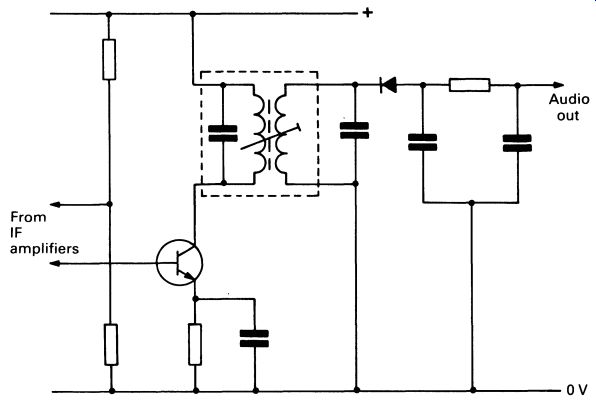
FIG. 20 an IF stage followed by a detector

There is one more feature that appears in all but the most rudimentary radio receivers, and that is the provision of automatic gain control (AGC). If a sensitive receiver is tuned to a powerful nearby transmitter, the signal may be so strong that it overloads the later IF amplifier stages, causing severe distortion of the sound. To prevent this, AGC is added. The idea and the circuit-is quite simple, and involves using a proportion of the rectified signal from the diode to control the biasing of the first IF amplifier transistor. A large signal at the detector diode lowers the bias potential at the base of the first IF transistor and reduces the gain-which, of course, reduces the output signal. With the right circuit values the receiver balances out with the correct output and bias levels.

To prevent the AGC responding to transient changes in the audio content of the signal (and increasing the gain during the singer's pauses for breath!), a large-value capacitor is placed across the AGC feedback line to delay the operation of the AGC by acting as a reservoir-the AGC then responds to the average signal level, averaged over a period as long as a couple of seconds.

An implementation of an AGC circuit is shown in Fig. 21 (refer also to Figures 19 and 20).

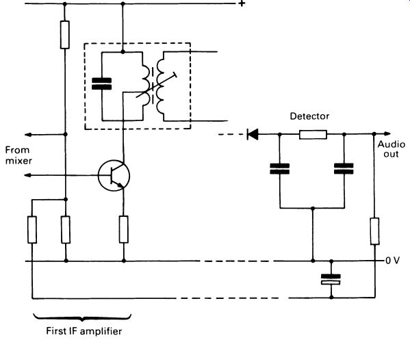
FIG. 21 application of feedback to provide automatic gain control

4. A PRACTICAL RADIO-CONTROL RECEIVER

It is quite possible to construct a working radio control receiver which, when used with the transmitter described at the beginning of this section, will have a range of up to half a mile. Commercially-designed radio control receivers generally use specially designed ICs that minimize the number of components required, .but this one uses circuits based on discrete transistors. It means that there are a few more parts, but it does have the big advantage that you can see how the circuit works, and find your way through the functioning of every part of the system. The complete circuit of the receiver, from aerial to output, is illustrated in Fig. 22.

This receiver is a little simpler than a broadcast receiver (and much easier to adjust) because it operates on a fixed frequency. The frequency is set by a crystal-controlled oscillator almost identical to the one used in the transmitter (and to the one in Figure 10.24), apart from a simplified bias circuit using just one resistor. In a broadcast receiver the local oscillator and the tuning circuit are adjusted in frequency together to preserve the correct intermediate frequency, which is then selectively amplified by the IF amplifiers. In the radio control receiver the requirement is for the tuning to be set to a single, very accurately determined frequency, which is why the more expensive crystal-controlled oscillator is used in preference to an LC oscillator.

The crystal is at a lower frequency than the crystal in the transmitter, differing from it by the selected value of the intermediate frequency, in this case 455kHz. The transmitter crystal was 27.095 MHz, so the required crystal for the local oscillator in the receiver would be: 27.095 - 0.455 = 26.640 MHz This produces the correct intermediate frequency when mixed with the incoming RF carrier. A signal received from a transmitter working on a slightly different frequency would produce an intermediate frequency higher or lower than 455kHz, which would not be amplified by the IF amplifiers and would therefore not produce an output.

The incoming radio signal is amplified by a JUGFET. This device is used in preference to a bipolar transistor because of its very high gate resistance, which maximizes the efficiency of the aerial tuning circuit (L2) that helps to reject powerful signals at unwanted frequencies. The output of the oscillator is transformer coupled to the source of the JUGFET (the signal does not need amplification), so that mixing of the radio and oscillator frequencies takes place. Following the mixer there are two IF amplifier stages. Bias for the transistors is obtained entirely from the AGC line --again, slightly simpler than the 'textbook' circuit in Fig. 21.

The detector stage incorporates a diode between the base and emitter, to rectify the input signal for that stage. The AGC voltage is derived from this stage. Finally, there is a d.c. amplifier fitted with low-pass filters to reject unwanted noise from the earlier stages.

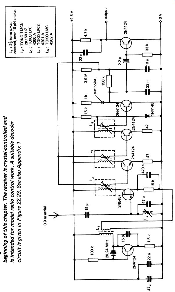
FIG. 22 the circuit of a complete superhet receiver; this is a practical design for use with the 27 MHz transmitter described at the beginning of this section. The receiver is crystal-controlled and is intended for model radio control work. A suitable decoder circuit is given in Figure 22.23. See also Appendix 1

FIG. 23

This circuit will work perfectly with the transmitter- -but as it stands the transmitter will be sending only the carrier, and there won't be any output! To tune the receiver, a modulated 27.095 MHz transmission is needed. A borrowed AM model control transmitter could be used, fitted with a 27.095 MHz crystal, but the transmitter described in this section can be used with a modulation system described in Section 22.

To tune the receiver, the 0.9 m aerial must be connected and arranged roughly straight. Connect a voltmeter to the collector of the detector transistor (marked 'test point' in Fig. 22) via a 4.7 k-Ohm resistor. Select a range reading around 5 V full scale. When the battery- ideally a 4.8 V nickel-cadmium accumulator- is connected, the meter should show little, in any, deflection. Switch on the transmitter with the aerial collapsed.

When the transmitter is moved close to the receiver, the meter will begin to show a deflection. Using a plastic trim-tool, adjust L2 for the maximum deflection, if necessary moving the transmitter away to keep the meter reading about 2.5 V. Now repeatedly adjust L3, L4, and L5 in turn to obtain the highest possible meter reading, if necessary moving the transmitter even further away; you may end up with the transmitter several meters from the receiver. When no further improvement can be obtained, the receiver is correctly aligned.

5. CONSTRUCTION PROJECT

Sufficient information has been given here (and will be in Section 22) to enable you to build the model control transmitter and receiver as a construction project. Although circuit layout is not particularly important, the printed circuit board designs given in Appendix 1 are recommended.

The designs are fully compatible with modern radio control practice, and can be used with commercially available servos (see also Fig. 23).

6. TELEVISION RECEIVERS

Having covered the principles of radio transmission and reception, it is now possible to consider the principles and practice of television. Even monochrome (black-and-white) televisions are extremely complicated in the details of their circuits, and television is a complete subject in its own right. In Mastering Electronics the systems involved will be explained, but without circuit details, except where this is essential to an understanding of the systems. To include a detailed study of television (and of various other topics, also) would be to make this guide at least twice its present size and cost!

7. MONOCHROME TELEVISION RECEIVERS

Most people now know that motion picture films produce the illusion of movement by presenting a rapid sequence of still pictures, each one slightly different from the one before it. The eye 'joins up' the pictures and interprets them as a single image in smooth motion, a phenomenon called 'persistence of vision'. Home movies (silent) show 18 frames of film (i.e. 18 pictures) every second. Sound movies shown 24 frames per second.

The movement on the television screen is created in exactly the same way, and the television transmission is sent out as a series of 'still' pictures, at the rate of 25 per second in the UK and many European countries, and at the rate of 30 per second in the USA and elsewhere. (The rate is actually half the frequency of the mains supply in the country in question. In the UK the mains supply is at 50 Hz, and in the USA it is 60Hz.) Central to the television system is the TV tube, illustrated in section in Figure 5.8 . The bright spot is made to scan the front of the tube continuously, in lines running across the screen, moving down from top to bottom in a pattern called the raster (see Fig. 24).

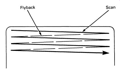
FIG. 24 television screen showing the raster.

The brightness of the spot is reduced to nothing during the right-to-left 'return' stroke, the flyback. In the UK the screen has 625 horizontal scan lines in the raster; it is slightly different in some other countries.

Unfortunately, a scan of this sort would produce flicker, even at 25 frames per second, whereas a motion picture film running at the same speed would not. The reason lies in the way the television picture is drawn from the top downwards, whereas the motion picture projector uncovers the whole of each frame virtually at once. To reduce the flicker, which has an odd appearance of running from the top down the screen, interlaced scanning is used, and the picture is produced in two halves, each taking 1/100 th of a second ( UK). The electron beam scans the screen as above, but only with 3121 lines. When it gets to the middle of the bottom of the screen (the 312-1/2 th line!) it returns to the middle of the top and scans the picture again, but between the first set of lines, 'interlacing' the second scan with the first. Using this technique makes the amount of flicker hardly notice able. Interlaced scanning is illustrated in Fig. 25, though with an 11-line screen instead of 625, to make the diagram clearer.

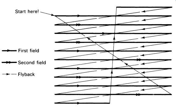
FIG. 25 interlaced scanning

It is important to realize that in a monochrome television the phosphor on the screen is completely homogeneous; the lines are merely a product of the scanning that produces the raster.

Two time periods are critical to the television: the time the beam takes to scan the width of the picture-the line frequency; and the time taken for one frame-the frame frequency. Two oscillators within the receiver generate these frequencies, and they are called, respectively, the line time base and the field time base. The line time base has to scan the screen 25 x 625 = 15 625 times every second, so has an operating frequency of 15.625 kHz, and the field timebase scans the picture 50 times every second (twice for each frame; remember the interlaced scanning), so operates at 50 Hz (the mains frequency--you will see why this is a good idea later). The timebases have not got to operate at about the right frequency, they have to work at exactly the right frequency, to scan the screen in exact synchronism with the cameras at the studio. For as the electron beam sweeps across the screen it is modulated so that the brightness of the screen is changed continuously to produce a picture. Fig. 26 shows how a picture is built up.

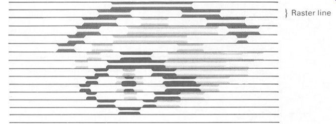
FIG. 26 the brightness of the spot forming the raster is modulated to provide pictures on the television screen

Clearly the timebases have got to be exactly in synchronism with the timebases of the cameras at the broadcast studio, or the TV picture will be chaotic, with no recognizable images at all. The transmitted signal therefore includes information about the timing of the line and field scanning, and circuits in the receiver extract this information and use it to synchronize the two timebases.

Every single sweep of the line timebase is triggered by a pulse in the signal received by the television. An RF carrier from the transmitter is modulated with a waveform corresponding to the brightness of the line of the TV picture. Fig. 27 shows part of this waveform, corresponding to two lines of the picture.

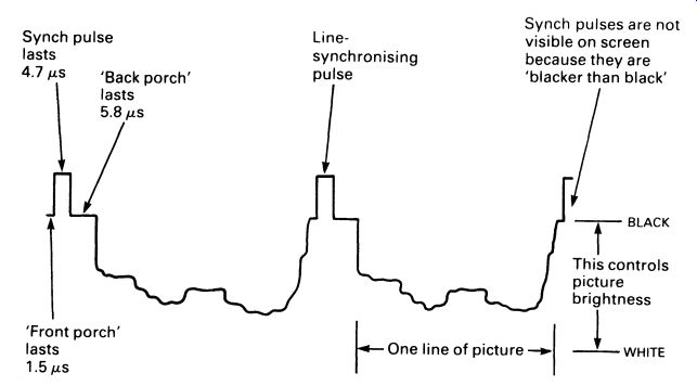
FIG. 27 the waveform of a television picture broadcast; this is the waveform that is recovered from the AM signal received by the television

Compare the waveform in Fig. 27 with the one in Fig. 28, which shows two lines of a picture consisting of four vertical stripes, progressively darker from left to right.

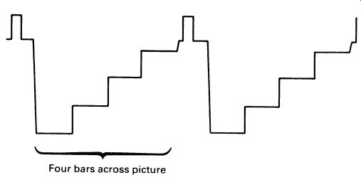
FIG. 28 two lines of a television picture showing four vertical bars of increasing density

The line-synchronizing pulses each trigger the line oscillator into a single sweep across the picture, or more commonly are used to synchronies an oscillator to run at a precise speed. Although in theory it would work to have an oscillator that is triggered for each line, in practice this would mean that any tiny interruption in the received signal would result in the loss of a synch pulse, and the loss of overall synchronization for the rest of that field.

At the end of each field there is a special series of line-synchronizing pulses that also trigger the field synchronization. The actual sequence is quite complicated and is shown in Fig. 29.

FIG. 29 the synchronizing pulse sequence at the end of each field

Following the last line of the picture in any particular field there are five equalizing pulses, followed by five field-synchronizing pulses, followed by another five equalizing pulses. The exact function of the equalizing pulses is subtle: suffice to say here that it makes the circuits in the receiver simpler. The five field-synchronizing pulses are detected by the receiver circuits-they are five times longer than 'ordinary' synch pulses-and trigger the next sweep of the field timebase. Once again, a synchronized free running timebase is used to prevent the picture collapsing entirely if the signal is lost momentarily.

Following the pulse sequence for field synchronizing there are a further 12.5 'blank' lines that are not used for the picture. These are put in to give the electron beam in the tube time to fly back to the beginning of the next field at the top of the picture. When all these various pulses and blank lines are taken into account, a total of twenty lines are 'lost' for each field, i.e. forty for each frame. For a television system like that used in the UK, having 625 lines per frame, only 585 lines actually appear on the screen.

A system diagram for the line and field scan of a television receiver is given in Fig. 30.

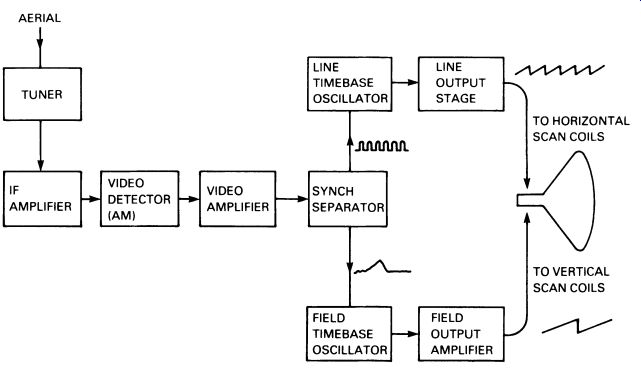
Fig 30 system diagram of the synchronization and scanning circuits of a monochrome television receiver.

8. TELEVISION SOUND

The signal for TV sound is transmitted on a completely separate carrier; in the UK it is 6 MHz higher in frequency than the carrier used for the vision.

The two carriers are amplified together in the receiver IF amplifier circuits, and then combined in a mixer. Since the sound is frequency modulated and the vision is amplitude-modulated, the result is a frequency modulated difference frequency, centered at 6 MHz, and carrying the sound.

This then goes its own way, being amplified separately, detected with an ordinary FM discriminator (phase-locked loop, etc.; see above), fed to an audio amplifier and finally to the speaker.

9. TELETEXT

The information used to update teletext systems in receivers equipped to show 'Ceefax' and 'Oracle' (in the UK) is transmitted in the form of binary code, a series of pulses, much more closely spaced than the line synch pulses. Teletext arrived after the television standards were all established, and made use of a feature included for other reasons-the blank lines following the field pulse sequence. The 'blank' lines are no longer blank, but are filled with the coded binary information. The teletext system selects the binary pulses and feeds them into a digital system that processes and displays the teletext information on the screen when required.

Only part of the teletext information is transmitted at any time, for it would be impossible to fit in the huge amount of binary code, even over 12-1/2 lines. The teletext system therefore includes a computer memory circuit that selects and holds the required information. Pressing the keys for a new teletext page makes the system 'look at' the pulses, each group of which begins with a code number (in binary) corresponding to a page of text. When the teletext system detects the number you have selected, which might take several seconds, it feeds the binary information into its memory, changing the picture on the screen. The picture then remains in the memory-and on the screen, if you want it-but is updated by the teletext system every time the selected number is detected in the binary coded information.

Complex circuits are used to mix teletext and vision, display different things on different parts of the screen, and to provide a 'newsflash' facility that puts information on the screen only when a change in content for a particular page is detected.

In theory, the amount of information that can be carried via teletext is unlimited, but the more different pages that are transmitted, the longer the delay in selecting a new page, as information for that page will come up less frequently.

10. THE COMPLETE TV RECEIVER

A system diagram for a complete TV receiver is shown in Fig. 31.

The only circuit we shall consider, even briefly, is the line output stage.

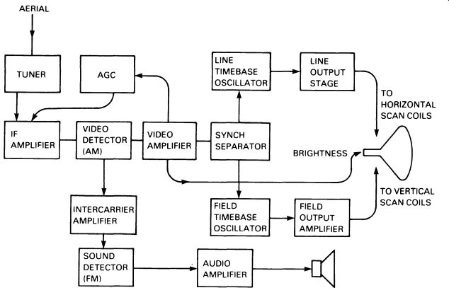
FIG. 31 system diagram of a monochrome television receiver.

This is the oscillator that provides the waveform required to make the electron beam in the tube scan the lines from one side of the tube to the other. As can be seen in Fig. 30, the waveform is a 'sawtooth'; the waveform is applied to the horizontal scan coils, and relatively high voltages are needed. The flyback has to be fast, and the voltage changes very abruptly. It is possible to make good use of this. In order to produce the high voltage necessary to drive the horizontal scan coils, a transformer is used, driven by the line oscillator. An extra secondary winding is put on the transformer, called the line output transformer (WPT), and with a large number of turns this winding can produce a very high voltage indeed, enough, in fact, to supply the final anode of the picture tube (see Figure 5.8 ). The line output transformer is therefore a vital-and dangerous-part of the power-supply circuits, as well as part of the line scanning system.

11. COLOR TELEVISION RECEIVERS

The problems facing the designers of the color television system were formidable. The television system was well established with monochrome receivers, and it was important that the color television system used would be cross-compatible. That is, a black-and-white receiver should be capable of receiving a color transmission and would reproduce it correctly (in black and white); and at the same time, a color receiver should repro duce a black-and-white transmission as well as a monochrome receiver.

The extra information required for the color receiver therefore had to be 'fitted in' round the existing signal, and in such a way that it would not interfere with the operation of a monochrome receiver. The color signal also had to be squeezed into the available bandwidth, which had been established as 8 MHz.

Since the eye is far less sensitive to color than it is to brightness, it proved possible to transmit the color information over a rather restricted bandwidth, so that the color on a color television is actually rather fuzzy. But if the brightness is controlled with a relatively wide bandwidth signal, giving a sharp picture in terms of brightness, the resulting picture is perfectly acceptable.

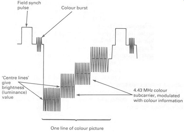
FIG. 32 the waveform of one line of a color television picture (the waveform is for a picture consisting of four vertical bars, like the one in Fig. 28)

Fig. 32 shows a waveform corresponding to one line of the same four vertical stripes illustrated in Fig. 28 above, but with color information added. The color signal is actually coded during the vision information period, and at first sight seems to be likely to interfere with a monochrome receiver. But remember that the frequency of the color signal--the chrominance waveform--is high, at 4.43 MHz, and would not be resolved by the circuits of the monochrome receiver, which would average the signal. The average is shown dotted in Fig. 32, and is obviously the same as the brightness waveform-called the luminance waveform--of the bars in the illustration in Fig. 28.

By means of a theoretically (and practically) complex method known as quadrature modulation, information about three colors can be obtained from the frequency-modulated chrominance subcarrier. (The waveform is called a 'subcarrier' because it is a carrier waveform, derived from modulation of another carrier of higher frequency.) The complete range of colors can be reproduced from these three color signals, as we shall see.

It is, however, necessary to have a 4.43 MHz reference oscillation, not only at precisely the same frequency as the reference oscillator back at the transmitter, but also exactly in phase with it (see Fig. 12 for a reminder about phase relationship). This technical miracle is achieved by means of a crystal oscillator in the receiver, synchronized in frequency and phase with a short (ten cycles) burst of the 4.43 MHz transmitted just after each line-synchronization pulse. The oscillator can be relied on to remain at the right frequency and phase for one line duration, 64 uS! The short burst of reference frequency is called the color burst.

Even with a system like this, slight changes in the transmitted waveform, caused by weather conditions, reflections from aircraft, etc., can cause phase errors between the color burst and the actual picture colors. The effect of this is a drift of the whole color spectrum towards red or blue--not desperate, but enough to notice. Despite this problem, this system was adopted in the USA, the first country to have a broadcast color TV network. The system is called the NTSC system, after the American National Television Standards Committee. (Opponents of the system claim that NTSC actually stands for 'Never Twice the Same COLOR', but this is not true.) The system adopted in the UK and many other countries, with the benefit of learning from the pioneers' mistakes, is known as PAL, which stands for Phase Alternation by Line. This overcomes the color shift of NTSC by the ingenious method of turning round the modulation system on alternate lines. COLOR shifts still occur, but alternate lines are changed towards blue and then red, and blue and then red, etc. The eye merges the colors and the overall impression is correct.

Very large color shifts still look odd. The effect is a bit like a multi colored venetian blind, so a modification of the PAL system, known as PAL-D was introduced. PAL-D actually adds the color signals of alternate lines electronically, by storing a whole line in a device called a delay line while waiting for the next line. The color on the screen is always the product of two alternately coded signals, and the result is effectively perfect color stability.

12. COMBINING COLORS

The information recovered from the transmitted signal is about three colors only, but it is possible to use the three colors to make every color in the visible range. In just the same way that the artist can make every color (if he wants to) by mixing primary colors, so the three primary colors of the color TV are mixed in different proportions to produce the whole range of colors. The three colors used are red, green and blue. Mixed together in equal proportions, these make white (white light is 'all the colors of the rainbow' mixed together), and other colors can be made by mixing two or three in different proportions. For example, green and red mixed together produce a bright yellow. This process is called additive mixing, and is not the same as the mixing of artist's colors, which is called subtractive mixing. The artist uses pigments that reflect only certain colors from the white light falling on them-they subtract colors. In the TV tube, colors are mixed-they are added together.

There are three factors that affect the picture on the screen. These are brightness, hue and saturation. Brightness is straightforward, and on the screen is controlled by the increase or decrease of all three colors simultaneously. Hue (color) is controlled by the balance of the three colors, as described above. Saturation refers to the 'strength' of the color, the amount of white light that is added to the basic color. Red, for example, is a saturated color. Pink is red mixed with white, and could be said to be a less saturated red. White light is not of course produced by the TV receiver, so saturation is in fact controlled by the difference between the brightness of the three primary colors; it is convenient to think of it as the color mixed with white, however.

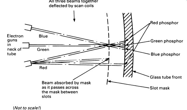
FIG. 33 principle of the slot-mask color television tube

13. THE PICTURE TUBE

The color TV picture tube is a development of the monochrome tube illustrated in Figure 5.8. The overall shape is the same, but there are three separate electron guns. In the most popular type of tube, the slot-mask tube, the three electron guns are arranged in a row, horizontally. The guns produce three electron beams, one for each color, and although the beams are all deflected together by the vertical and horizontal scan coils, the brightness of the beams can be controlled separately.

All three beams therefore scan the front of the tube together, to produce a raster. Obviously, it is not possible to have colored electron beams, so the color is produced in phosphors on the front of the screen.

Phosphors can be made almost any color, and the right shades of red, blue and green can be produced easily, if expensively. The raw materials for the colored phosphors actually contribute significantly to the price of a color TV tube.

The trick is getting the 'red' beam to affect only the red phosphor, the 'blue' beam to affect only the blue phosphor, and the 'green' beam to affect only the green phosphor. This is done by simple geometry. Fig. 33 shows the system diagrammatically, viewed from the top of the tube. All three beams together deflected by scan coils ; Beam absorbed by mask as it passes across the mask between slots ; Red phosphor Green phosphor Blue phosphor Glass tube front lot mask

The slot-mask is fixed firmly in place behind the tube, and the relation ship of the positions of the slots and of the phosphor strips on the back of the tube is such that the 'red' electron beam can fall only on the red phosphor, etc. Fig. 34 is a perspective sketch of the tube, from which you can see that the slots are quite short, and are 'staggered' to produce an interlocking pattern. This arrangement is used because it is physically strong-great rigidity of the mask is clearly important-and because it gives a reasonably large ratio of 'slots' to 'mask'. The more transparent the mask is in this respect, the better, for electrons which hit the mask rather than go through the slots are just wasted power, and serve only to heat the mask. The larger the slots can be made in relation to the mask, the brighter the picture will be.

The slot-mask principle is used in the popular precision in-line (PIL) tube, which is manufactured complete with scan coils as a single unit. This, together with extremely sophisticated scan-coil design, produced in the first place with computer-aided design techniques, has led to a tube that is very simple to use, all the most critical alignments having been built in at the manufacturing stage.

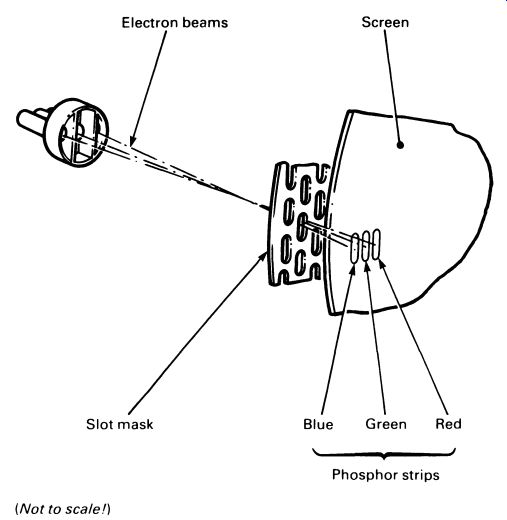
FIG. 34 perspective drawing of a slot-mask color TV tube

A variation of the slot-mask tube is the Sony Trinitron tube. This uses an aperture-grill instead of a slot-mask. The aperture-grill consists of vertical strips, like taut wires, with complete vertical phosphor stripes in different colors printed on the back of the tube. The Trinitron® tube has very good mask transparency and gives a good picture brightness. The Trinitron® tube also includes an improvement to the electron gun system, in which the three electron beams all pass through a single common point in the neck of the tube, so that they all appear to originate from the same point. This makes adjustments of the scanning system easy, and improves the focus (the sharpness of the picture on the screen). Earlier color TV receivers used 'delta-gun' tubes, which had the three electron guns arranged in a triangle, and circular holes in the shadow-mask tube. These tubes are not now used in new receivers, as they are rather difficult to adjust and give poorer picture brightness for a given beam power than either the PIL tube or the Trinitron.

There is not space here to give more than the briefest glance at color television receivers. The circuitry is, in both theory and in practice, very complicated, and extensive use is made of special-purpose integrated circuits to reduce the 'component count' and to make the receivers easy and cheap to manufacture. In real terms a color television costs less that its monochrome counterpart of thirty years ago, and gives incomparably better results.

Television servicing, especially color television servicing, is highly specialized, and should never be attempted by the inexperienced or untrained. The voltage on the final anode of a color receiver will be more than 25 kV, and is usually lethal.

Before leaving the subject of color TV, get hold of a pocket magnifying glass, and take a close look at the surface of a color TV tube, first with the receiver turned off, then with it turned on.

QUESTIONS

1. What is meant by wavelength?

2. What kind of oscillator is used for radio control applications? Why?

3. Why are germanium diodes, as opposed to silicon diodes, often used in the detector stage of radio receivers?

4. Describe amplitude modulation, and compare it with frequency modulation.

5. Draw a circuit for a 'crystal set' radio receiver, and describe how it works.

6. What are advantages of the superheterodyne receiver?

7. Why do radio receivers and transmitters usually have to be 'trimmed', or adjusted, before they can be used?

8. Why do television systems use interlaced scanning?

9. Describe the functions of the television line and field synchronizing circuits.

10. Which part of the television's circuits generates the EHT supply for the final anode of the cathode ray tube?

11. Which colors are used to make the whole range of visible colors in a color television tube?

12. Sketch the internal layout of a color TV tube, showing how the electron gun assemblies produce the relevant color on the front of the tube.