Reviewed by CH
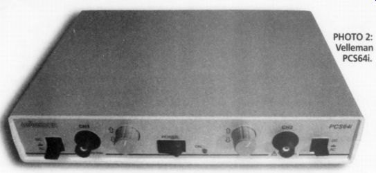
PHOTO 2: Velleman PCS64i.
PCS64i Digital Storage Oscilloscope for PC; $400 US, Velleman, Legen Heirweg 33, 9890 Gavere, Belgium; US Distributor, Velleman-Kit, 7415 Whitehall St., Suite 119, Ft. Worth, TX 76118, (817) 284-7758, www. Velleman.be.
The Velleman PCS64i, an 8-bit PC-based DSO, uses an interface unit that contains analog signal-conditioning circuitry and a dedicated analog-digital converter (ADC) for each of its two analog channels. The software provides both DSO and FFT functions, as well as a separate transient signal recorder (TSR).
The Interface The interface unit, shown in Photo 2, is 8.75"W x 1.75"H x 6.5"D. The front panel has two BNC jacks for independent two-channel operation, as well as a power switch and LED indicator. Each channel has an input switch to select AC or DC coupling or GND, and a vertical position pot.
The box connects to the LPT1 printer port with a supplied data cable. No other LPT port address is available, so you will need a switch box to access your printer if you don't wish to keep switching cables. A 9V DC plug-in adapter powers the PCS64i. You must power up the box before you start the program or connect scope probes to a live signal. Software communicates with the box to enable the computer to act as a two-channel oscilloscope display.
The PCS64i is designed to use 1x or 10x scope probes (an available option that was not provided with the test unit).
Other options are a rechargeable battery pack and a carrying case.
Both DOS and Windows 3.1/95 soft ware are provided. I did not evaluate the DOS version since its capabilities are limited, including the lack of 64 Msample/ sec oversampling.
The WinDSO software installation is simple and straightforward, requiring only 1MB of free hard-disk space. The installation program makes an additional subdirectory for data and graphics files.
An uninstall program is also provided.
Since Velleman makes three other PC based instruments, you must enable the PSC64i from the Option menu before you can access the PCS64i box.
The four-language owners' manual is well-written, with numerous diagrams to aid in learning the PCS64i. Circuit schematics, the PC-board layout, and ser vice-calibration information are provided in the back.
Circuit Description
The PCS64i was the only one of the three DSO units I reviewed that was furnished with a schematic. The entire unit is contained on a multilayer PC board with surface-mount components. The 9V DC power input is converted to +5V DC. A constant-current regulator is provided to charge the optional Ni-Cad battery pack.
Two identical input channels are provided, so I will I describe one channel of the I § analog input circuit. The input switch selects AC or DC coupling. An additional GND position opens the BNC connector and also grounds the scope-input amplifier. Each analog input signal is connected across a conventional 11 M ohm (in parallel with) 30pF
R-C attenuator, as in any scope.
Reed relays under software control select one of three taps at 1M, 100k, or 10k.
The tapped signal is input through 100k to a cascoded JFET circuit whose gate is protected by clamp diodes (the maximum input voltage is 100V peak, AC + DC). The output from the JFET is sent to an AD811 high-performance, current-feedback, video op amp whose gain is selected by two more reed relays under software control. The vertical position pot introduces a DC offset into the inverting input circuit of the op amp. The output from the AD811 goes to an emitter-follower that drives the analog input of a TDA8703 8-bit DAC. Data is stored in an 8K x 8 SRAM.
The digital portion of the unit is controlled by a pair of programmable logic devices and some high-speed CMOS glue logic. The PCS64i interfaces with the computer LPT1 port by means of 15 optoisolators with 3000V isolation. (For some reason the optoisolator devices are not shown on the schematic, but do appear on the PC-board layout drawing.)
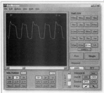
FIGURE 2: 5SMHz square wave at 32MHz sample rate.
DSO Screen
The program boots in the DSO mode and presents the familiar oscilloscope format with 8 x 10 graticule (see Fig. 2).
I found the scope didn't quite fit in my display, so I reduced the VGA-display's vertical dimension. This left a 2" black border around the desktop when I exited WinDSO. You can set the vertical input for each channel from 10mV/div to 5V/div. If any part of the input signal exceeds +4 divisions, the display clips and shows a horizontal line until the signal level comes back into display range. The time base can be set from 0.1us/div to 100ms/div. The selected time/div and volts/div for each channel appear just above the scope display.
Operation of the DSO is completely intuitive. You select the time base and volt age buttons using the mouse. The screen update is quite fast, although, like most 8 bit DSOs, the waveforms have a rather jagged appearance. You can improve this by selecting the S/L smoothing function, which is most effective for frequencies below 5MHz. The S/L button works only on the 0.5, 0.2, and 0.1us time bases.
You can select the reticule grid to be bright or dim.
You can save any waveform on the screen in bitmap (bmp) format, or copy and paste it to another document (the DOS software saves in TIFF format).
There is no way to print directly from the DSO, FFT, or TSR modes. You must save the data or screen-graphic images, and run them in their separate programs. The data format is an ASCII table that lists the 4096 data points and the time- and volt age-step scaling factors for the data. A bitmap image opens the PC Paint pro gram, where you can print it. I was able to cut and paste images into a number of Windows programs, such as Word, Power Point, and Excel.
The manual states that "if after leaving the program the stored pictures and/or ASCII text are not to be lost, they must be transferred from the Data directory to another directory. If this is not done, the next set of measurements will overwrite these files." I did not find this to be a problem, since you are allowed to assign a filename to any saved image. Perhaps it is a problem in the DOS software, where filenames are automatically assigned.
Independent Channels
The two channels are truly independent, with 4096 records stored per channel. If you use only one channel, the data list for the unused channel lists the cursor position with no signal. You do not drop to half the memory or half the sample rate when you engage the second channel.
Each input is rated for a generous 100V peak (AC + DC) max, and is not fuse-protected. Excessive input voltage can dam age the PCS64i interface box, but it has 3000V of optical isolation from the computer port, and there should not be any subsequent damage to your computer.
I tried a number of signals on the DSO to assess its limits. Two full cycles of the 1kHz square wave from my function generator displayed reasonably well, with some least significant bit (LSB) toggling on the horizontal portion of the signal, and the leading edges were slightly rounded. The vertical portion used three data points for the full transition.
With the time base set for 0.1ms (one cycle displayed), I was able to zoom the stored 1kHz image between 10us and 0.5ms per division. Beyond that, there was no display at all. From an initial 0.2V/div, I was able to zoom from a nearly flat line at 5V/div to screen clipping at the upper and lower limit at the lower V/div settings. The response time when switching between time base or voltage ranges was less than one second.
I decreased the square-wave frequency to 100Hz, 10Hz, and 1Hz, adjusting the time base accordingly, and the waveform was square in these ranges. From 10-500kHz, the leading edges, with one or two cycles on the screen, showed some random peaking using the default 32 M-sample/sec rate. At the 5-MHz limit of my function generator, the square wave display is shown in Fig. 2. (Figure 2 is a Print-Scrn capture. The remaining scope figures (except for Fig. 8) make use of the program's bitmap save.) The use of 64 M-sample/sec (Fig. 3) results in a more accurate and ragged waveform.
When I applied smoothing with the L/S button, the square wave took on a more sinusoidal appearance (Fig. 4), so you must apply it carefully.
The function-generator triangular waves had nice sharp points on the peaks, with a slightly notchy appearance along the transitions.
Accuracy Check
To check accuracy, I fed the PCS64i a low-distortion 6.4V RMS 1kHz sine wave from the oscillator of my HP339A distortion test set, with the DSO set to 5V/div and 0.2ms/div. I used the markers to mea sure the + and -peaks of the sine wave and the time span of two zero crossings.
The peak-to-peak dV was very close to 18V (the markers are mouse-dragged, and have no step-movement capability, so resolution depends on your "mouseability").
The dT reading was very close to 1ms.
The RMS readout was 6.27V RMS, about 2% lower than the actual voltage. This is reasonably accurate-probably better than you could achieve with an analog scope. The marker functions are very handy for these measurements.
Next I increased the time base to check for aliasing, which creates illegitimate frequency components when the sampling frequency is less than the Nyquist frequency, or twice the signal bandwidth. Aliasing became apparent at 2ms/div where the width of one or more of the 20 displayed cycles started to vary.
Amplitude modulation occurred above 5ms/div, and there were some dots scattered at the original peaks of each sine wave. At 50ms/div, aliasing was in full bloom, with the dT zero-crossing markers for the 1kHz signal reading 33ms--equivalent to a 30Hz sine wave.
I selected 1V/div and reduced the sine wave amplitude to the lowest level where the LSB toggled. Then I decreased the V/div until the V RMS display was within 5% of the actual voltage, which was 3.9mV on the 10mV/div range. This result is consistent with the accuracy of the 8-bit ADC converter used in this DSO.
Complex Waveforms
To see how well the PCS64i handled complex but repeatable waveforms, I sampled the 19kHz + 20kHz CCIF wave form from my intermodulation distortion (IMD) meter. While not noticeable in Fig. 5, there were some sample dots scattered at the peaks. The more complex 9kHz + 10.05kHz + 20kHz MIM signal is shown in Fig. 6. Since I could not apply smoothing at 0.2ms/div, the display is much more jagged than it would be on an analog scope.
I decided to display the chaos of a pink noise signal, which shows up on an analog scope as electronic cotton candy. The DSO capture was much more orderly, a victim of significant aliasing and under sampling. You have to be very careful with any DSO, even a high-performance one. What you see isn't necessarily true.
For the final DSO test, I ran a 1kHz, 4V RMS sine wave from the function genera tor through my HP339A. The upper _A-01447-6) ow wave trace in Fig. 7 is the fundamental, which measured 0.57% THD+N. The lower waveform is the residual distortion signal (not to scale) after passing through the -100dB notch filter. You can clearly see the second harmonic, along with the lower-amplitude fourth.
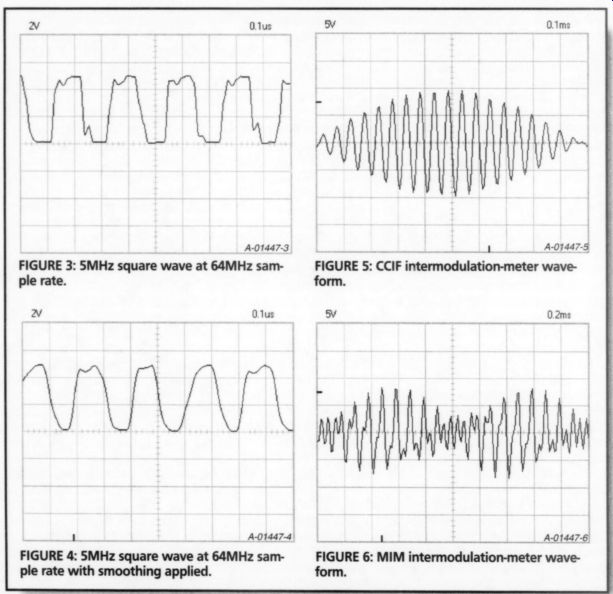
FIGURE 3: 5MHz square wave at 64MHz sample rate.
FIGURE 4: 5MHz square wave at 64MHz sample rate with smoothing applied.
FIGURE 6: MIM inter-modularization-meter waveform.
To test the math functions, I fed CH 1 a 1kHz sine wave and CH 2 a 2kHz sine wave (not synchronized). Second-harmonic summing was clearly visible using the CH1 + CH2 or CH1 - CH2 function.
A familiar two-lobed Lissajous pattern developed in the x-y plot mode. The math functions work in both real time and with stored waveforms.
Triggering Modes
Professional oscilloscopes offer
-------
I used the one-shot mode to check the triggering sensitivity, and was able to trigger at 500ns, the narrowest single pulse my function generator can provide.
FFT Screen
The FFT display is that of a spectrum analyzer, with vertical magnitude and horizontal frequency as shown in Fig. 8.
The vertical input uses the same V/div ranges as the DSO mode. The frequency-range se lector sets the maximum frequency, which extends over 16 horizontal divisions, from 800Hz-16MH The spectrum is displayed from zero to the selected frequency. Since only ten divisions are visible, the horizontal-position scroll bar is used to access the six hidden divisions. There are also four zoom but tons that can expand the stored horizontal display x1, x2, x4, or x 8 times. Frequency increments can be in either linear or log format.
---------
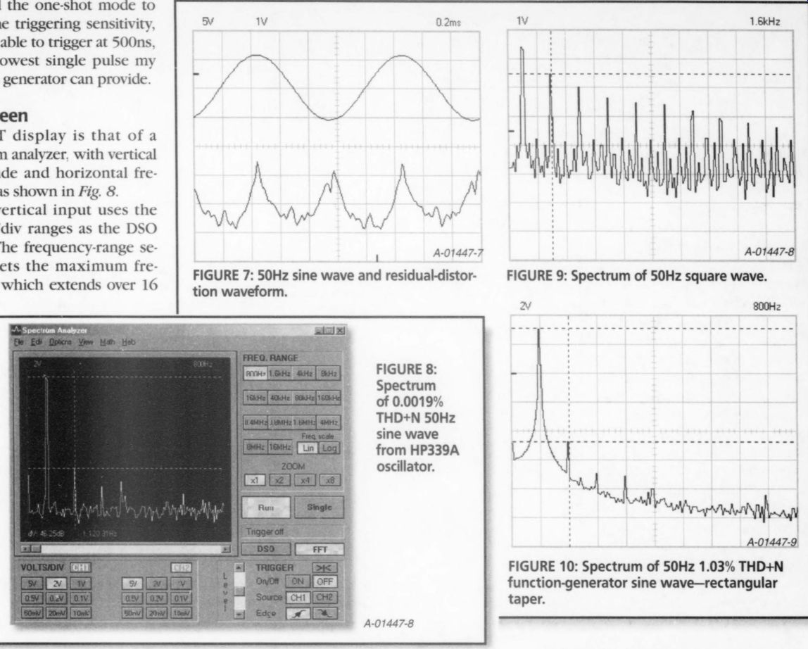
FIGURE 7: 50Hz sine wave and residual-distortion waveform.
FIGURE 9: Spectrum of 50Hz square wave.
FIGURE 8: Spectrum of 0.0019% THD+N 50Hz sine wave from HP339A oscillator.
FIGURE 10: Spectrum of 50Hz 1.03% THD+N function-generator sine wave-rectangular taper.
The Options menu offers five FFT weighting filters, or tapers:
Rectangular, Bartlett, Hamming, Hanning, and Blackman.
Three measurement markers are provided, one less than DSO mode. The horizontal markers measure V or dV, reading out in dBV (0dBV = 1V), and the vertical marker reads frequency. The Velleman manual says to use AC-coupling in the FFT mode, probably in order to eliminate any false even-order harmonics. The triggering circuit works on signal amplitude just like the DSO mode.
The FFT display screen has a range of 80dBV, which changes with the V/div range. At the 10mV/di of the V/div range. At 10mV/div the range is from -114dBV to -34dBV, and at 5V/div the range is from -60dBV to +20dBV. I decided to use the 2V/div range where possible, with 3V RMS input signals, which gave me a theoretical range of -68dBV to +12dBV. You must be careful that the V/div range you select does not clip in the DSO mode. Otherwise, you will introduce the harmonics that result from the clipping into the spectrum. I ran a baseline of the 2V/div noise floor by selecting GND on the input switch in the 800Hz range. The peaks of the noise floor proved to be -58dBV for CH 1 and -60dBV for CH 2. The unit's DAC is rated for -55dB harmonics, all components, and 7.1 effective bits, so this unit is certainly in the ballpark. In addition, there are power-supply artifacts at 120Hz (-45dBV) and 240Hz (-52dBV), which may be caused by the plug-in power supply, given the modest --25dB supply-voltage ripple-rejection rating of the DAC, and may disappear when you're using the optional battery power pack.
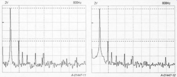
FIGURE 11: Spectrum of 50Hz 1.03% THD+N function-generator sine wave-Bartlett taper.
FIGURE 12: Spectrum of 50Hz 1.03% THD+N function sine wave-Hamming taper.
FFT Testing
You can use only one channel at a time for FFT, so I chose CH 1 for the tests. I applied a 3V RMS 50Hz sine wave from the HP339A test oscillator function (0.0019% THD+N). I set the upper V marker on the 50Hz peak and used the lower V marker to measure dV in dB (actually dBr, or relative dB).
While there were no apparent 50Hz harmonics, which is as it should be, the noise floor was ~63dB, which is far above the actual -94dB for this frequency. As you can see in Fig. 8, the predominant frequencies on the display are the 120Hz, 240Hz, and 480Hz signals, rep resenting harmonics from the PCS64i's own power supply.
The next test was an easy one, applying a 50Hz square wave to the FFT. Since a square wave is an infinite series of odd harmonics whose amplitude is the fundamental peak times the inverse of the order of the harmonic (5 of the third, 5 of the fifth, and so on) the THD+N for a square wave is 33%. The results using the 1.6kHz range were perfect down through the 13th harmonic. After that, the measured data was one or two dB lower than the ideal until it hit the noise floor at the 23rd harmonic. Figure 9 shows the first nine harmonics.
There is also some evidence of even order harmonics, which should not exist in a pure square wave. They may result from nonlinear amplification in the analog input circuit, sampling jitter, or non-symmetry in the function-generator output. I don't consider them to be a problem.
Next I set the function generator for a 3V RMS 50Hz sine wave. This pseudo sine wave is derived from the triangle wave by using a diode-resistor sine shaper network, and it measures 1.03% THD+N on the HP339A. I recorded the FFT spectrum with each of the five weighting tapers (also called filters or windows), the purpose of which is to ensure that the time-domain data starts and stops at the same data value, and that the function in between is smooth.
Recall that amplitude clipping can cause false harmonics to appear in the spectrum display. This can also happen if the data is not periodic in time, that is, if it does not start and stop at zero. The taper is designed to act as a frequency-domain filter, and its width and attenuation characteristics trade off the three variables of accuracy, selectivity, and noise floor.
Taper Measurements
Figure 10 is Rectangular, Fig. 11 is Bartlett, Fig. 12 is Hamming, Fig. 13 is Hanning, and Fig. 714 is Blackman (Black man-Harris). The Rectangular taper pass band is steep and narrow, but has significant side-lobe ripple in the reject bands.
This manifests itself as a widening of the "skirt" around the center frequency, which could "hide" low-level nearby frequency components, but it has good amplitude accuracy.
The Hanning taper is not as steep in the passband, but has less ripple in the reject bands, with a narrower skirt, and may be less accurate in depicting a very pure waveform or transient events. The Hanning is also commonly used to mea sure random noise. The Blackman taper is more accurate than the Hanning, and has the fastest rolloff. It is very selective, at the expense of amplitude accuracy.
I applied two equal-magnitude 250Hz sine waves that were combined in a low distortion, unity-gain, inverting, summing op-amp circuit. This placed the spectrum peak at mid-screen on the 800Hz range. I then increased one of the frequencies until two distinct peaks were just visible.
All five tapers separated the two signals with a AF of only 5Hz. I continued to in crease one frequency until the separation extended fully down to the noise floor.
The Blackman taper AF for this condition was only 6Hz, with the Hanning close behind at 8Hz. The Bartlett taper required 20Hz, and the Hamming taper 40Hz. The Rectangular taper was not fully separated at the base of each skirt until the two sine frequencies were 110Hz apart.
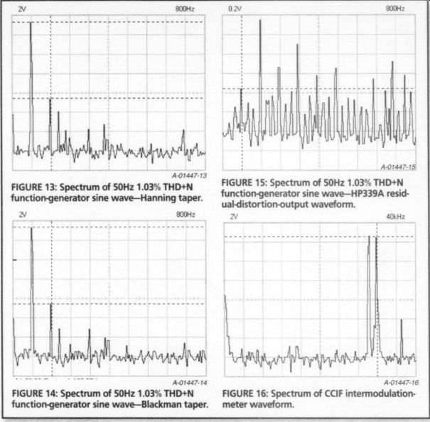
FIGURE 13: Spectrum of 50Hz 1.03% THD+N function-generator sine wave-Hanning taper.
FIGURE 14: Spectrum of 50Hz 1.03% THD+N function-generator sine wave-Blackman taper.
FIGURE 16: Spectrum of CCIF intermodulation meter waveform.
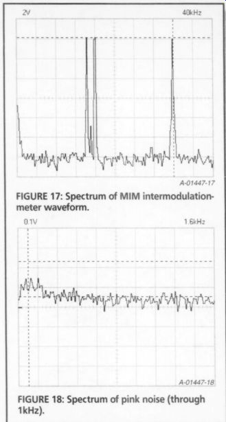
FIGURE 17: Spectrum of MIM intermodulation meter waveform.
Since the Hanning taper is the most common among FFT instruments, I used it to measure the spectrum levels, using the FFT program markers (Fig 13). You must disregard the multiples of 120Hz, since they occur in response to the PCS64i power supply. The noise-floor limit was about --60 dBV.
THD-Signal Spectrum
I also performed a test described by Lynn Olson and Matt Kamna ("Sound of the Machine: The Hidden Harmonics Behind THD," Glass Audio 4/97, p. 1), which records the spectrum of the THD signal at the residual output of a distortion meter. In this case I passed it through the HP339A distortion-test-se fundamental notch filter and captured the monitor output. There is much more harmonic detail in Fig. 75 than in Fig. 13. Using the Olson/Kamna method, 1 gained an apparent 29dB of headroom (based on normalizing the level of the second harmonic), thus making the PCS64i much more useful.
Figure 15 also shows the spectrum lines to be progressively less than the 100Hz spacing of the horizontal-axis grid lines as the frequency increases. This is because the actual sine frequency was a bit on the low side. The PCS64i showed good frequency accuracy as long as I took care to avoid aliasing.
Figure 16 is the spectrum of the 19kHz + 20kHz CCIF inter modulation-meter waveform at 3V RMS. The FFT is set to the 40kHz range here. The harmonic at 23kHz is of no consequence in the intermodulation test. The meter has a very narrow +80dB bandpass filter at 1kHz that looks only for the 20kHz-19kHz intermodulation difference product that results M from nonlinear amplification.
The more complex 9kHz + 10.05kHz + 20kHz MIM wave form in Fig. 17 has no visible harmonics.
The spectrum of pink noise using the 1.6kHz range is shown in Fig. 18. Pink noise has a 1/f characteristic, in that the energy decreases with frequency. This is visible even over the limited frequency range shown in the screen display.
Transient Signal Recorder Screen
This screen is a separate program. You must first close the Oscilloscope/FFT program and run the Transient Recorder pro gram. A transient signal recorder is simply an oscilloscope with a very slow time base. The PCS64i extends from 20ms/div to 2ks/div. The full 16-division horizontal time span is shown on the display.
I tested the REC mode by recording the AC line at my test bench using some simple signal-conditioning circuitry.
Using a full-wave rectifier and filter, I measured the output of a 12.6V AC step down transformer, with a bleed resistor/divider that gave me a time constant consistent with the sample time. I set the divider to give me a DC level equal to 10% of the AC-line amplitude.
I connected another 12.6V AC step down transformer to my HP339A and set it to measure 60Hz distortion. I bread boarded a precision full-wave rectifier circuit (National Semiconductor Application Note AN-20) to convert the AC monitor output (after the HP339A fundamental notch filter) into a DC voltage proportional to THD+N.
I monitored the AC line amplitude with CH 1, and used CH 2 to monitor the power-line THD. I set the REC on 500s/ div and let it run. This gave me a record a little over two hours long. It is interesting to see how many little blips and dips occur in the AC line over this time period, including one spike above 127V RMS.
The distortion ranged between 2.9% and 3.2%.
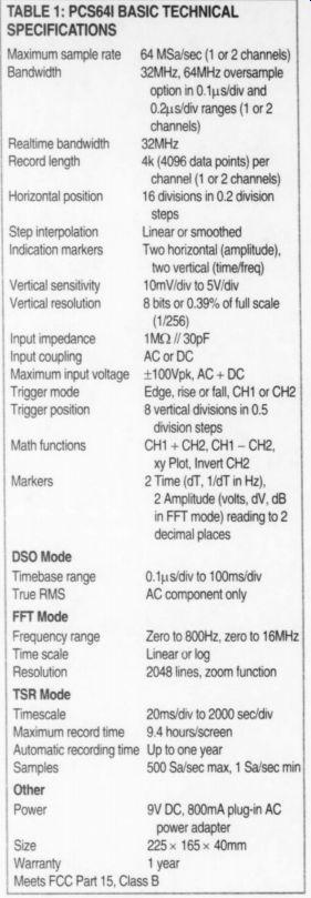
TABLE 1: PCS64I --BASIC TECHNICAL SPECIFICATIONS
Maximum sample rate
Bandwidth 64 MSa/sec (1 or 2 channels) 32MHz, 64MHz oversample option in 0.1us/div and 0.2us/div ranges (1 or 2 channels)
Real-time bandwidth 32MHz
I Record length 4k (4096 data points) per channel (1 or 2 channels)
I Horizontal position 16 divisions in 0.2 division steps
Step interpolation
Linear or smoothed
I Indication markers Two horizontal (amplitude),
I two vertical (time/freq)
I Vertical sensitivity 10mV/div to 5V/div
Vertical resolution 8 bits or 0.39% of full scale (1/256)
I Input impedance 1M ohm // 30pF
I Input coupling AC or DC
Maximum input voltage +100Vpk, AC + DC
I Trigger mode Edge, rise or fall, CH1 orCH2
I Trigger position 8 vertical divisions in 0.5 division steps
I Math functions CH1 + CH2, CH1 - CH2, xy Plot, InvertCH2 Markers 2 Time (dT, 1/dT inHz), 2 Amplitude (volts, dV, dB in FFT mode) reading to 2 decimal places
I DSOMode
I Timebase range 0.1us/div to100ms/div
True RMS AC component only FFT Mode
I Frequency range Zero to 800Hz, zero to 16MHz
I Time scale Linear or log
I Resolution 2048 lines, zoom function
I TSRMode
I Timescale 20ms/div to 2000 sec/div
I Maximum record time ~~ 9.4 hours/screen
I Automatic recording time Up to one year
I Samples 500 Sa/sec max, 1 Sa/sec min
I Other
Power 9V DC, 800mA plug-in AC power adapter
Size 225 x 165 x 40mm
Warranty 1 year
I Meets FCC Part 15, Class B
Conclusion
While its accuracy and resolution are not comparable to those of a modern high performance oscilloscope, the PCS64i easily outperforms the $10,000 professional two-channel DSOs that were introduced in the late 1970s, and it provides lots of additional useful features. At $400, it is a good value for the hobbyist and anyone else with a high-performance analog scope who needs some DSO capability for troubleshooting. The PCS64i has a higher frequency response than most 8-bit DSOs, and the optical isolation protects your computer from dam age, which is a major advantage.
Also see:
On The Mechanics of Tonearms, Part 1