by Richard C. Heyser
TRANSIENT RESPONSE, like the weather, is something many people like to talk about, but, darn few do anything about. Audio has done something about transient response by providing a measurement of the time spread which a speaker imparts to a dynamic signal. It is known as the energy-time test. First, let's consider the nature of transient response and what it means to the illusion of sound in reproduction.
Transient sounds are sudden changes. They are the "now" sounds that give liveness and sparkle. Transient sounds, of the type to be discussed here, are over and gone in a very short time and hence are generally un-pitched to the listener. A mathematical analysis of them, however, usually shows a broad frequency distribution of sound energy that may be many octaves wide and extend upward beyond the limit of audibility.
Transient sounds are the opposite of steady-state sustained notes.
What does poor transient response in a speaker mean to the reproduction of sound? For one thing, it generally means a loss of realism. The bite of brass, attack of strings, and snap of percussion are all affected. Quite often we sense that all the frequencies are there but the reproduction is indistinct. The sibilants of an otherwise good stereo image of a choral group may tumble over each other in a cascading waterfall of sound and destroy the illusion of depth.
How do we test for transient response? There are many tests but the most meaningful derive from an impulse as a source. Before it was finally accepted as a respectable generalized function, the impulse was usually regarded by mathematicians as a pathological entity that didn't quite fit into the scheme of things, even if it gave correct answers. A true impulse, for the purpose of speaker testing, would be an infinitely short duration, infinitely large voltage spike which at the moment of application would have a known constant energy. No one is going to generate that in any laboratory, you can be sure. But we know that if you could, the speaker would generate a sound called the impulse response. The impulse response will persist long after the impulse is over, just as a bell rings down after a sharp hammer blow.
The usefulness of the impulse response is due to the fact that any signal, no matter how complicated, could be duplicated by a continuing progression of impulses. In other words, if you know the response to an impulse, you have everything to know about the response to any arbitrary signal. And now you have a direct handle on the description of a transient.
Finding the Impulse Fortunately, we don't have to try to generate an impulse for testing. We can compute the response. This neat little trick is made possible because the impulse response of a device is mathematically identical (almost everywhere, as the strict mathematician would insist) to the Fourier transform of the true steady-state frequency response.
This is exactly how we go about it.
We start from the true frequency response, which must include the phase as well as amplitude, and compute the impulse response. We're not home free yet, because the conentional impulse response is a signal that generally looks like a series of overlapping oscillatory wiggles. While all the transient information is there, the waveform is almost unintelligible unless you are an expert at deciphering the story it tells.
What we have done is gone a step further and computed the total energy density represented by the impulse response. But a little history is in order.
The true frequency response is a complex quantity which has a magnitude as well as a phase angle. It wasn't too long ago that most people rebelled at the idea of loudspeaker phase response, but now most accept that reality. The thing we compute from the frequency response is, in fact, the time response of the loudspeaker. Time response also has a magnitude and a phase, and what Audio plots is the magnitude of the time response. To put it mildly, this is a whole new idea in audio measurement. While we also compute the phase of the time response, we have elected to plot only the magnitude because it is a measurement you can understand with very little practice.
So what happened to that wiggly line known as the impulse response? It has been absorbed into the energy density plot. The energy-time plot is the true magnitude of the envelope of the impulse response. The impulse response fits into the energy-time response like a hand in a glove, but now the energy response fills in all the spaces between the peaks of the impulse response. What has happened is that the time response may either be represented in rectangular coordinates with an in-phase and quadrature component or in polar coordinates with a magnitude and angle. The impulse response is the in-phase rectangular component, and since in our case it represents instantaneous sound pressure, it contains the information relating to potential energy density of the generated sound. The quadrature component, once you compute or measure it, contains information relating to kinetic energy density. We actually compute this and then, when we convert the rectangular data into polar format, the magnitude is now related to total energy density since it properly contains kinetic and potential energy density in the proper proportions.
Two other considerations are needed before we close off this technical summary. First, we deliberately restrict our computation to cover only those frequencies from d.c. to 20 kHz.
This simplifies the computation and is reasonable from the standpoint that sounds above 20 kHz are not generally considered in loudspeaker measurement. The true Fourier transform requires using all frequencies from d.c. to infinity. The result of using a restricted band of frequencies is that a perfect time response is spread from the infinitely narrow impulse into a broader peak and, in fact, will have time sidebands extending both prior to and following the true time of impulse. This leads to the second consideration because simply chopping off the frequency spectrum as if it were a rectangle gives a (sin t)/t time pulse which dies off too slowly to be of value in evaluating speaker transients.
We therefore weight the frequency response with what is known as a Hamming response prior to conversion from frequency to time. This gives a slightly broader time response for a perfect loudspeaker but knocks down the clutter very well.
Using the Data
Now, let's consider how to use the data. Suppose we had a perfect loudspeaker situated in front of a microphone such as sketched in Fig. 1.
Directly below the sketch of microphone and loudspeaker we have a plot of received energy versus time.
The perfect loudspeaker would cor respond to a hump of energy centered at one meter distance, corresponding to about 3 mS air path delay.
The spike is the impulse we would get if infinite frequencies were considered while the blunter peak is what we get from using 20 kHz.
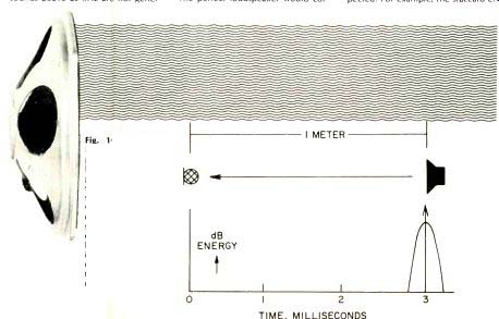
Fig. 1-A perfect loudspeaker reproducing an ideal band limited impulse will cause a short burst of sound energy which appears to come from the spot in space occupied by that loudspeaker. This is the acoustic signature of perfection in transient response.
If, as in Fig. 2, some reflecting surface causes sound to scatter toward the microphone, the two signals will be picked up. One signal is the direct sound due to the actual speaker, while the second is reflected sound due to the image speaker. This then shows up as two energy humps.
Now let's put our speaker in a box.
In typical fashion we will cut a hole in the front panel and mount the speaker on the backside, creating a small resonance cavity due to the finite panel width. Other physical considerations are as shown in Fig. 3. The first sound heard is the direct sound shown as (a). Early reverberation produces the multiple humps (b). The spherical sound wave expanding from the loudspeaker will diffract from the molding trim, or any edge discontinuity, first at (c) then at (d). Sound from the back of the cone might reflect from the rear and reappear as (e).
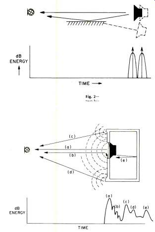
Fig. 2-A scattering surface will cause two bursts of energy to be heard from
an otherwise perfect loudspeaker.
Transient response is now degraded by this added echo.
Fig. 3-Mounting an otherwise perfect loudspeaker in a box causes degradation of transient response by creating sound scattering heard as echoes and reverberation. These transient robbing sounds are measured by the time smear of energy which an actual speaker imparts to a perfect band limited impulse. By calibrating the arrival time and amount of these scattered sounds it is possible not only to tie them to the speaker system structure which causes them, but identify the amount of pace smear which is imparted to otherwise perfect transient sounds.
This direct tie to the physical structure of a loudspeaker system can tell a great deal about the sound to be expected. For example, the staccato effect of reflection in Fig. 2 is clearly in evidence in most loudspeakers. Usually the scatter giving rise to this is so short in time that all we sense is a "smear" in detail. If you want to determine what such an effect sounds like, walk up close to a reflecting surface, such as a hard wall, and listen to some percussive sound, such as a typewriter. (It helps to plug the ear opposite to the wall when doing this.) Not a very accurate portrayal of the sound of the typewriter, is it?-particularly when you can turn around and hear what it should really sound like.
A desirable plot, then, from the standpoint of excellent transient response, will have a narrow primary energy arrival with very few peaks following this and all the later peaks much lower in level than the primary signal. This type of loudspeaker will reproduce short transient sounds realistically. Any broadening of the primary energy or appearance of subsidiary reverberant energy will dull the performance to some extent.
Because this one-meter energy time measurement is obtained directly from the one-meter frequency response, it is possible to correlate structural problems with frequency response problems. A loudspeaker that has a good frequency response when mounted on a large surface in an anechoic chamber can have a poor response when placed in a "busy" enclosure. Some manufacturers, however, use the measurements made anechoically with a large baffle in their literature and ads, rather than the response of the actual system that would be used in the home. A response aberration such as (c) in Fig. 3 may be loosely tied back to frequency response by looking at that portion of the frequency range which has the distance between (a) and (c) as an integral fractional wavelength.
We usually restrict the energy-time measurement to one curve for simplicity. The curve we do give can tell the best story about transient response for the first few milliseconds, which is probably the most meaningful part of the story. Because the tweeter and midrange units cover a broader frequency range than the woofer, their contribution to energy for this time must be correspondingly greater, and the physics of reproduction says it must be. One piece of information that is not shown is the pitch contribution of each source of energy. The pitch information would be contained in the equivalent time-phase plot. It may happen that the timbre of response (c) is different than that of direct sound (a). In truth, the "timbre" of any given loudspeaker is made up of the net contributions of each of the parts, a and b and c and so on.
There are several things to look for in the plot Audio provides. We use a logarithmic energy density scale, calibrated in dB, to make certain features stand out. A time response that has an exponential decay, such as the ring down of a strong resonance, will show as a straight line fall off of log energy versus time. The slope of this decrease is related to the "Q" of the peak. Multiple reverberation, which is a discrete form of exponential decay, will show as (b), peaks which are joined by a straight line reverberation characteristic. In fact, the reverberation time may be obtained by extrapolating the curve to-60 dB relative to the first peak.
Energy Decay
A logarithmic plot of energy density also allows for greater visibility of transient distortion than the conventional linear plot of impulse response.
Coherent signal fragments 40 dB down are clearly audible but would require an enormous linear plot to be seen. Remember that in order for a second sound to be judged "half as loud" as a first sound it need only be down between 6 and 10 dB in measured level. Some of these early reverberations which are 20 dB down from the principal peak are not inaudible by any means.
Experience has shown that the form of many of the aberrations in speaker transient distortion show more readily in a log plot. One "form" that repeatedly shows is the characteristic of diffraction due to a diffuse surface.
The shape of direct energy sources, such as (a), are relatively smooth at peaks, whereas diffraction effects, such as (c) are generally irregular.
When a cone loudspeaker is under test, the first signal energy you may see is due to sound coming off the edge of the cone. This is usually an energy peak on the rising slope of the first main peak. Elastic waves in a speaker cone consist of a combination of shear and compressional components and propagate faster than sound in air. These are first to reach the front of a speaker, and if the cone surround is not a perfect absorber, they will "launch" a sound wave from that point as they reflect back toward the voice coil. Normally this is a very inefficient mode, and the energy is very low. However, the propagation of the elastic waves down the cone can efficiently launch pressure waves as it travels, an effect ingeniously capitalized on by Lincoln Walsh in his now famous driver. Many direct radiator speakers have poor polar and transient response for the first few tenths of milliseconds because of these sound waves caroming off domes, whizzers, and the cone itself. This will show clearly in the energy-time plot.
We realize that the concept of the time response of a speaker is a whole new ballgame to many people and is probably a bit confusing if all you ever considered before was steady-state frequency measurements. However, once you begin to use such data and get accustomed to both time and frequency measurements, the tendency is to get hooked and not want to go back to only frequency measurements. You then realize you need both types of data to fill in the whole story of loudspeaker performance.
Audio has introduced the plot of energy density as a function of time not because it is the only possible one, but because if you must give only one measurement of time performance, this is perhaps the most meaningful for evaluating speaker sound.
(Audio magazine, 1976)
Also see:
Making Records/Ralph Cushino (June 1976)
Equipment Profiles: E88 "Eclipse" Model 2240 Electronic Crossover/Leonard Feldman; Garrard Model 86SB Turntable/George W. Tillett (July 1976)
Audio in General (Departments): Audioclinic/Joseph Giovanelli; Tape Guide/Herman Burstein; What's New In Audio ; Audio ETC/Edward Tatnall Canby ; Behind The Scenes/Bert Whyte (July 1976)
= = = =