Television and FM Receiver Alignments [How To Understand and Use TV Test Instruments (1953)]

INTRODUCTION

The Federal Communications Commission in their regulations covering television broadcasting limit the video frequencies which may be transmitted to a maximum of 4 mhz. This means that the television signal may contain all video frequencies from 0 up to and including 4 mhz. All broadcast station equipment is designed to pass all 4 mhz. It may happen from time to time that full use is not being made of this bandpass, possibly because of the character of the signal or misadjustment of the equipment. However, with all transmitter units in proper operating condition, 4 mhz will be passed.

In the receiver, conditions are somewhat different. Manufacturers have found that acceptable pictures can be obtained with a bandpass as low as 3 mhz (2.5 mhz on small screen tubes) and many of them have taken advantage of this to effect economies at the expense of picture quality. The serviceman will have to take cognizance of this fact when he aligns a receiver in order that he does not waste time trying to obtain a 4 mhz response from a circuit designed for 3 mhz. The serviceman's job is to return the set to its normal operating condition; he is not charged with the responsibility of redesigning the circuit, no matter how badly this is needed in some instances.

Information concerning the bandpass of a television receiver is also useful in detecting trouble.

A circuit or system that should possess a 4 mhz band pass may properly be suspected of containing trouble if it indicates only a bandpass of 2.5 mhz. This knowledge is important although, unfortunately, it is not as readily available as it should be.

The wide bandpass characteristics of television receivers coupled with their higher. operating frequencies make them somewhat more critical in alignment and adjustment than AM radio or FM receivers and it is quite common to find sets which are poorly or improperly aligned. This is perhaps the greatest single defect which is present in today's millions of television receivers.

The technique of properly aligning a television receiver is not a simple one to acquire. Not only must the technician be familiar with television circuitry and operation, but what is just as important, he must be completely familiar with the instruments he uses. It is perhaps as much on this latter point as the former that many servicemen fall down and it is the purpose of this section to aid the serviceman to acquire mastery of this skill as much as possible.

The alignment of a television receiver is most conveniently performed in the following order:

1. Sound Detector

2. Sound IF transformers

3. 4.5 mhz trap or take-off coil (in Intercarrier receivers)

4. Video IF traps, if any

5. Video IF transformers and coils. (This includes mixer transformer.)

6. Overall video IF

7. RF Section

Some manufacturers specify a somewhat different order but the general approach re mains substantially the same. In the paragraphs to follow, the type of equipment which is needed to accomplish the alignment of each portion of a TV receiver will be considered together with specific instructions on how this equipment is connected and how the adjustments are made. In all instances, typical circuits will be employed.

SOUND DETECTOR

Figure 1. The Manner In Which the Response Pattern of a Foster-Seeley Discriminator Would be Obtained.

The sound signal broadcast by a television station is frequency modulated and consequently the sound detector must be an FM detector. In common use today are two types of FM detectors: The ratio detector and the Foster-Seeley discriminator. While both circuits differ considerably in design, they do possess the same "S" type of response and this is the indication which the service man is seeking when aligning these circuits.

A typical Foster-Seeley discriminator is shown in Figure 1. The demodulated audio output from this circuit appears between point A and ground ( or chassis) and if we connect the vertical input terminals of an oscilloscope between these two points the circuit response pattern will appear on the screen. The sweep or frequency-modulated signal from the generator would be fed into the system at the grid of the last sound IF amplifier. If a ratio detector is being employed in the receiver, the instrument set-up remains substantially the same (see Figure 2). In both circuits the oscilloscope vertical input terminal connects to the point where the audio signal leaves the FM detector; the oscilloscope ground lead attaches to the receiver chassis.

Let us look closely at both the sweep generator and the oscilloscope because that is primarily what we are interested in here. Prior to obtaining any circuit response pattern on the scope, we would set its controls so that a scanning trace was visible on its screen. The procedure for doing this was described previously in Section 4. The vertical gain control would initially be set at mid-position or slightly beyond, permitting the scope to produce a sizeable pattern with moderate input signals. The vertical attenuator, if such a control is available , might initially be set to its most sensitive position. (When you are working with a scope which is not too sensitive, it might be best to set the vertical gain control also for maximum amplification.)

Figure 2. The Manner in Which the Response Pattern of a Ratio Detector Would be Obtained.

The sweep generator should be connected with its "hot" output lead going to the grid of the last sound IF amplifier and its ground connecting to the receiver chassis. The generator frequency would be set at the sound IF carrier value--say 21.00 mhz if this happens to be its frequency. The sweeping range required is 1 mhz or perhaps somewhat more although it is not recommended that this extend beyond 2 mhz at the most. The RF output control could be turned to its maximum position initially in order that some indication will be obtained on the scope screen if the circuit is operating. It has been found that it is better, at the start, to have both instruments going full blast and then to tone each down as needed rather than to work up to the proper level. The brute force approach appears to be better suited for the beginning technician perhaps because the appearance of some indication is a quieting and reassuring factor psycho logically. (Not to be overlooked is the low signal output of many low priced sweep generators. These units frequently have to be run "wide open" at all times.) Thus far nothing has been said about the insertion of a marker signal and indeed nothing should be done along these lines until a normal indication is obtained on the scope screen. By keeping the number of complicating factors as low as possible, the chances of confusion are minimized.

The sweep generator is now set up to apply its signal to the circuit under test and the oscilloscope is connected to receive whatever output is obtained from the FM detector. However, before any power is turned on in the receiver, there are several other steps to be taken. First, a lead should be connected from the horizontal s weep voltage terminal of the sweep generator to the horizontal input terminal of the oscilloscope. This will feed in a 60-cycle sine wave driving voltage to the oscilloscope and cause the scanning beam to move instep with the signal generator's sweeping voltage. A ground lead should connect both instruments although if the two are properly grounded through the receiver chassis, the additional connection may not be necessary.

Next, set the oscilloscope controls so that this sweeping voltage drives the beam across the screen in place of the instrument's internally generated saw tooth voltage. If the scope possesses its own 60-cycle sine wave deflection voltage and phase control (such as the units shown in Figures 15, 16, 22, and 39 of Section 4), the driving voltage from the sweep genera tor will not be required. In this case, you would simply set the scope controls to provide the desired sine wave sweep.

Another step to be taken before the alignment is begun is to prevent any signal other than that developed by the sweep generator from reaching the circuit under test. To do this, pull out one of the prior sound IF tubes. If the set is of the transformerless type and the tube filaments are series connected, tube, pulling would open the filament circuit. In this case signals can be prevented from reaching the discriminator by unsoldering a grid lead on a prior tube or by placing a short circuit from grid to ground on this tube. Frequently the short will suffice although sometimes opening the circuit becomes necessary.

You are now ready to turn on the equipment and proceed with the alignment. Permit the set and the instruments to warm up for about 10-15 minutes to be sure that each has reached a stable operating condition. At the end of this time the oscilloscope should carry some indication of a response curve if the instruments and the circuit are operating normally.

The output of the generator now should be turned down as far as possible and still provide a usable indication on the scope screen. Also, the vertical gain control on the oscilloscope should be adjusted until the pattern covers at least one half of the screen. Make certain the amplifiers in the oscilloscope are not being over loaded. A good test for overloading is to watch the pattern as the sweep generator output is alternately increased and decreased. If the height of the pattern on the screen varies in step with the generator output, no overloading is occurring. But if the pattern re mains stationary through all or part of the generator output variation, then overloading is occurring . Another indication of overloading is an S curve possessing flat-topped ends.

Figure 3. When You First Obtain a Response Pattern on the Screen, You Will Most Probably Have a Dual Trace.

Figure 4. When the Phase Control has Been Properly Adjusted, the Two Patterns of Figure 3 Will Blend Together, as Shown.

Figure 5. Response Distortion When the Discriminator Primary is Misadjusted.

Figure 6. Response Distortion when the Secondary Slug is Misadjusted.

At this point the pattern on the screen may or may not be the looked-for S response curve. If it is, then, of course, the work to follow will consist simply in determining whether it is on-frequency and making such minor adjustments as may be necessary to improve its linearity. The more natural assumption and the one more likely to occur is that while some sort of curve will be obtained on the screen, it will not have exactly the desired S shape. Let us see what can cause this and what steps can be taken to correct it.

Probably the first thing you will notice about any indications on the scope screen is the fact that there are two patterns. This stems from the phase difference between the 60-cycle driving voltage in the sweep generator and the 60-cycle sweeping voltage which is driving the scanning beam in the oscilloscope.

To bring the two patterns together, rotate the phase control.

The next step is to bring the response pattern to the desired S shape. See Figures 3 and 4. Deviations from this form may arise from two sources: Circuit misalignment or a generator that is not on frequency. Misalignment of the circuit as a cause of waveform distortion is well-known. Thus, when the primary of the discriminator transformer is misadjusted, the S curve takes on the appearance shown in Figure 5; when the secondary trimmer or slug is incorrectly positioned, the curve appears as shown in Figure 6.

With the appearance of an S curve, you are now ready to apply the marker signal for specific frequency identification. Take a good look at the S curve before the marker signal is applied; any appreciable change in curve shape thereafter will be due to excessive marker signal or to marker generator loading on the circuit. Neither of these conditions is desired and both must be carefully avoided.

MARKER SIGNAL INSERTION

The method of inserting the marker signal depends upon the equipment used. Where the sweep generator contains its own marker generator (such as the units shown in Figures 24 and 26 of Section 3), insertion of the marker simply means turning the marker oscillator on, setting it to the freq u enc y desired, and then slowly and gradually increasing its output until a marker pip appears on response curve on the scope screen.

Some sweep generators, while they do not generate their own marker signal, do contain provision for receiving the marker signal and combining it with the sweep signal. (See Figure 19, Section 3.) The marker signal would be applied to the proper terminal (and ground) and then its amplitude increased until the pip became visible on the screen.

Finally, there are many s wee p generators which do not have any provision for receiving the marker signal and when these units are employed, the marker signal must be introduced separately into the test circuit.

There are a number of ways of effecting marker signal insertion and the more common methods will be outlined here. Whatever the method, however, the precautions indicated above mu st be carefully ob served, otherwise not only will the marker signal be useless, but worse still, it will distort the response curve and prevent the serviceman from properly aligning the circuit.

1. Probably the simplest method of mark e r insertion is to connect the marker ground lead to the receiver chassis and then clip the marker "hot" lead directly onto the sweep generator's "hot" lead. This places the out puts of both generators in parallel.

Great care must be observed when using this method, however, because the shunting effect of the marker generator can readily affect the sweep generator out put to such an extent that the response curve is swamped or distorted. If this is found to happen, the disturbing effect of the marker generator can frequently be reduced or eliminated by using an isolating resistor between the "hot" lead of the marker generator and the point where it connects to the sweep generator output clip. A resistance value of 25,000-75,000-ohms will usually be sufficient.*

2. The marker signal may be inserted at the grid of a tube located before or after the point where the sweep signal is applied. If the marker generator is connected between grid and ground of a stage which is located prior to the point where the sweep signal is applied, then the marker generator lead may be connected directly to the grid of this tube# without the use of an isolating resistor. However, if the marker generator is connected to the grid of a stage through which the sweep signal is passing, then an isolating resistor (25,000 - 75,000 ohms) should be employed as a precautionary measure.

--------------

*The reader is cautioned against using an excessive value of isolating resistor. This can cause marker displacement on the response curve and lead to a false conclusion concerning frequency indication of the steeper portions of the response curve.

If a DC voltage (with respect to ground) is present on the grid, insert a .01 mfd isolating capacitor in series with the generator "hot" lead.

------------

Figure 7. The Marker Signal Need Not Necessarily Pass Through the Circuit Being Aligned in Order to Serve its Purpose.

Of course, where there is but one stage between sweep generator and oscilloscope, as in Figure 2, then the marker generator must be connected either at the same point as the sweep generator or at a prior stage.

An interesting fact with regard to marker insertion is that the marker signal need not necessarily pass through the stage being aligned in order to serve its purpose as an identifying agent. However, the marker signal must pass through the detector with the signal from the test circuit. To illustrate this point, consider the adjustment of circuit A in Figure 7. The sweep generator is connected so that its signal will pass through circuit A. The marker generator, on the other hand, is not injected into the system until point B where it combines with the out put of circuit A. Rectification of the signal then occurs at the detector, after which it is fed to the vertical input terminals of the oscilloscope. ( In Section 5 special marker generators were described wherein it was not necessary to pass the marker signal through the test circuit or its detector at all.

These units may be employed here in addition to the other methods described.)

3. The foregoing methods have dealt with direct insertion of the marker signal into the circuit. Usually just as effective and frequently less disturbing on the response curve is the indirect insertion of a marker signal. This can assume such forms as merely positioning the hot lead of the marker generator near the circuit under test or clipping the lead onto the body of a capacitor or resistor in that circuit or system. Since the body is composed of some insulating material, direct electrical contact with the circuit is avoided. However, by radiation of the signal from the lead clip plus some extraneous capacitive coupling, the signal reaches the test circuit, combines with the sweep signal and appears on the oscilloscope screen.

Another effective method is applicable to those circuits where the tubes possess shields. Simply lift the shield up until it is no longer making contact with its grounding base and then tilt the shield sideways slightly until it rests on the glass of the tube. If this is done carefully, the shield will be supported by the tube envelope and not make contact with the chassis.

Now clip the hot lead onto the tube shield and sufficient signal will radiate from the shield to the tube elements to serve as a marker signal injector. See Figure 8.

If you encounter trouble keeping the tube shield from sliding down and making contact with its grounding base, insert a small wad of paper between shield and tube.

An alternative method of marker injection, known as the "chassis" method,* is illustrated in Figure 9. The "hot" and ground leads of the marker generator are both connected directly to the receiver chassis, with the clips spaced approximately 6 to 8 inches apart. Position the clips on the chassis sothat they st r add 1 e the sweep generator injection point.

The lead signal voltages set up strong circulating ground currents in the receiver chassis which couples the marker signal into the circuit under test.

Irrespective of the method employed, always be on the alert against swamping the response curve by the marker signal. Never use more marker signal than is necessary.

Figure 8. Signal Injection by Clipping "Hot" Lead From Generator Onto Tube Shield. Make Certain Tube is not Touching Chassis or Other Ground Points.

*Suggested by the engineers of Precision Apparatus Company, Elmhurst, Long Island, New York.

Figure 9. The" Chassis" Method of Injecting a Marker Signal. Courtesy Precision Apparatus Co., Inc.

Figure 10. With a Blanking Control in the Sweep Generator, One of the Two Traces can be Converted into a Base or Reference Line.

Figure 11. A Double "S" Curve Produced When the Scope Beam is Deflected by a 120 Cycle Saw-Tooth Voltage.

Figure 12. When a 60 Cycle Saw-Tooth Deflection Voltage is Used in the Oscilloscope, The Screen Presentation Will Appear as Shown.

When the equipment has al. been set up and the circuit adjusted, the S curve and the marker pip should be visible on the screen. Some difficulty is sometimes encountered in locating the pip when it is moved along the steep linear section of the curve. One suggestion* for overcoming this is to reduce the sweep width control setting until only the center portion of the S curve (with its "pip") is visible on the screen. (The center frequency of the sweep generator may have to be readjusted as the sweep range is reduced in order to keep the center portion of the response curve on the screen.) When this is done, the expansion of the central portion of the discriminator curve produces a more pronounced "pip". The pip observed at the center of the "S" curve differs from the usual marker indication in that the actual center of the pip is re presented by the straight line portion of the "wiggly" line. This is due to the fact that discriminator output voltage is zero at the exact center IF. The double trace response curve, in which the two traces are brought together by means of the phasing control, is the type of curve that most service men will be working with. However, some s wee p generators contain a blanking control and with it one curve may be eliminated and a base or zero reference line substituted in its place. See Figure 10. Where this facility is available, it should be employed be-cause the reference line can be especially helpful in FM detector alignment.

A single trace ( without any base line) can also be obtained when the oscilloscope contains provision for beam blanking during the retrace portion of the cycle.

ALTERNATE "S" CURVE

There is still another method for presenting the "S" curve and this is shown in Figure 11. Here the oscilloscope is utilizing its internal saw-tooth deflection voltage operating at a frequency of 120 cycles per second. This means that during one-half of the sweep generator cycle, one S curve is traced out, then the scanning beam moves quickly back to the left-hand side of the scope screen and traces out the other S curve during the second half of the sweep generator cycle . Stabilization of the trace can be achieved either by setting the oscilloscope on line sync or by using the internal sync position. Some technicians prefer this method of discriminator alignment and many manufacturers recommend it. However , it does not insure any greater ac curacy than the previous methods and so it becomes a matter of personal preference.

A precaution that must be observed when using the saw-tooth oscillator of the oscilloscope to move the beam across the screen is that its frequency is close to 120 cycles. If the rate is reduced to 60 cycles, then the pattern of Figure 12 will be obtained.

Note that what you have here are two S curves back to back. Assumed identifying frequencies have be en included to help illustrate how this sort of presentation is obtained. In one complete sweeping cycle in the sweep generator, the band of frequencies are swept across twice. In other words, if the band sweep is 1 mhz and the frequency range covered extends from 24 to 25 mhz, then the generator output will go from 24 mhz to 25 mhz and then from 25 mhz back to 24 mhz again.

The beam in the oscilloscope is traveling forward throughout all this time, tracing out first the curve produced by the 24 to 25 mhz sweep and then the curve resulting from the 25 to 24 mhz sweep.

If the oscilloscope scanning frequency drops down to 30 cycles, four S curves strung out in a line will be seen.

When a variable frequency marker pip is employed with the presentation shown in Figure 11, its action will differ somewhat from that observed with an S curve obtained by using a 60-cycle sine wave deflection voltage. This, too, can be confusing unless the technician understands how the curves of Figure 11 arc produced. In the curve of Figure 4, only one pip will be seen as the marker frequency is varied because every point on this curve represents a different frequency. But now consider the double trace in Figure 11. The frequencies re presented by one curve are duplicated ( in reverse position) on the other curve. When a marker signal is introduced into this arrangement, one pip will appear on each curve at its proper point. Thus, let us say that the marker signal frequency is set at 24 mhz. Then one pip will appear at the 24 mhz point on one curve and one pip will be seen at the 24 mhz point on the other curve. If we raise the marker frequency gradually to 25 mhz, the pip on the lower curve will move to the right ( which is towards the 25 mhz point on this curve) and the pip on the other curve will move toward the left ( or to wards its 25 mhz point). The two travelling pips will meet at 24.5 mhz and blend into one if the two S curves cross at this frequency.

Figure 13. Sweep Generator Unbalance May Prevent Perfect Blending at all Points.

Figure 14. Two Curves Vertically Displaced From Each Other. See Text for Explanation.

ADDITIONAL CAUSES OF CURVE DISTORTION

In dealing with response curves which are presented on an oscilloscope screen, there are certain variations that the serviceman will encounter which can cause him some unnecessary trouble unless he is familiar with their cause. Non-linearities in the sweep generator output can produce a pattern in which the two curves will not perfectly blend with each other at all points. If the phase control is set so that blending is achieved at the righthand side of the curve, then the curves may not superimpose at the left. See Figure 13. This slight unbalance will have no effect on the alignment and the serviceman can proceed as if he had only one curve. Note that over the section where the two curves do not blend, neither will the markers (when they reach this region). Occasionally a condition will be found where the trace and retrace are essentially duplicates of each other but are more or less evenly displaced vertically.

See Figure 14. This is due to hum in the detector, or hum picked up by the response curve cable* or isolating resistor. In general, this condition is not normal and the cause of it should be determined (heater cathode leakage, insufficient filtering of the B+, poor grounding of generator or oscilloscope cable or receiver chassis, etc.). Placing your hand on the cable shield, on the test instruments, or on the receiver chassis should have no effect on the response pattern. If it does, poor grounding is indicated.

It sometimes happens that vertical jitter of the response pattern or multiple tracings is caused by the vertical circuits in the receiver itself. To determine whether this is so, simply remove the vertical oscillator or vertical output tubes.

Another source of confusion is an S curve on a screen which is 1800 out-of phase with the curve shown in the manufacturer's manual. See Figure 15.

If the oscilloscope has a phase reversal switch, then the situation can be "corrected". In the absence of such a switch, the alignment can be carried out with the reversed curve . As discussed previously, the polarity of the curve seen on the screen is primarily determined by the number of vertical amplifiers in the oscilloscope plus the position of the take-off point in the receiver. It has nothing to do with the alignment condition of the circuit under test.

----------

* Pick-up cables of the coaxial type (RG-59U or RG 11 U) are recommended for the oscilloscope. Cable length should not exceed three or four feet to prevent the build up of input capacitance to excessive values.

-------------

Figure 15. Two Curves 180° Out of Phase With Each Other. This is Generally Caused by Number of Vertical System Amplifiers in Oscilloscope.

ALTERNATE METHODS OF FM DETECTOR ALIGNMENT

Alignment of Foster-Seeley discriminators and ratio detectors c an be carried out by using an RF signal generator and a VTVM. The signal generator would be connected to the grid of the IF amplifier tube preceding the detector. Where the VTVM would be connected depends upon the type of detector circuit employed. If we consider the Foster-Seeley circuit first, then the initial VTVM connection would be made between point B and chassis, as indicated in Figure i6. It might be advisable to insert a 10,000 ohm isolating re s is tor between the VTVM pr ob e and point B. The RF generator is now set to the sound IF value (say, 21.00 mhz) and then the primary slug of the discriminator transformer, T1, would be adjusted for maximum indication of the VTVM. The lowest DC voltmeter range of the meter should be used, reducing the output of the signal generator to keep the needle on scale.

The transformer primary is now in adjustment and the secondary winding is tackled next. For this, the VTVM probe is switched to point A. The secondary winding slug is now adjusted until the meter reading is zero. Rotating the slug in one direction from the zero point should produce a positive meter reading while rotating the slug in the opposite direction should produce a negative reading. The correct setting for the discriminator slug is at the zero point.

To facilitate the observation of this zero point, a number of vacuum-tube voltmeters have a center zero reading scale. See Section 1. With these instruments, the meter needle is in the center of the scale (at zero) when the discriminator secondary winding is adjusted correctly. Off resonance is indicated by the meter needle swinging to the right or left of this zero mark.

Where your VTVM does not possess a special center zero reading scale, one of two methods can be employed to determine when the discriminator secondary is in balance. In one method, you would carefully adjust the secondary slug until the meter read zero. Then the "Function" switch would be turned from +DC to -DC. If there is no voltage reaching the meter, the needle will remain at the zero mark. However, if there is some slight unbalance and a small negative voltage is present, the needle will deflect. If this happens, adjustment can again be made, bringing the needle back to zero. The process can be continued until a switch from one polarity to the other does not deflect the needle.

The second method is known as the "False Zero" method and consists initially in using the "Zero Ad just" knob of the VTVM to purposely swing the needle to some point on the meter scale (using the lowest DC scale). Let us say that the point chosen is 1 volt (on a 0-3 volt scale). 1 volt now becomes our new "Zero" point because we have disturbed the meter balance to this extent. (Any new "zero" point could have been chosen.) Now, with the receiver in operation, and the VTVM connected between point A and ground, the secondary slug of T1 is adjusted until the meter needle is at 1. Turning the slug in one direction should swing the needle above 1; turning it in the opposite direction should bring it below 1.

Note that we have established our own zero point at 1. The meter will read 1 when it is not receiving any external voltages. A positive applied voltage will cause the meter needle to swing above 1 * and a negative applied voltage will force the meter needle below 1. Thus, when the discriminator secondary is balanced, no voltage should be present between point A and chassis and the meter needle should be at 1.

* provided the "Function" switch is in the +DC position.

This "False Zero" method is just as effective as a center zero scale and may be used on all VTVM's not possessing the center zero scale.

The discriminator is now aligned and generally this is as far as most servicemen go. However, it might not be amiss to make one more check to determine whether the central portion of the S-curve is linear. This is carried out by swinging the RF generator frequency 50 to 75 khz above and below the center IF frequency and noting whether equal frequency shifts above and below the center frequency produce equal (but of opposite value) voltage readings on the VTVM. Linearity of the S-curve is as important to the faithful reproduction of a program as the adjustment of any of the receiver stages. Unfortunately, many servicemen overlook this test when using a VTVM and an RF generator. They cannot ignore curve linearity when aligning the discriminator visually.

In aligning ratio detector circuits, the method of approach is altered somewhat. The RF signal generator is still connected to the grid of the IF amplifier tube preceding the detector. However, be cause of circuit differences, the VTVM is initially connected between point Band chassis. See Figure 17.

The primary slug of T1 is then adjusted for maximum meter indication. This done, the VTVM probe is then switched to point A and the secondary slug of T1 rotated for zero on the VTVM. As .before, the zero point is located between positive values on one side and negative values on the other and any of the zeroing methods previously described can be employed here.

The Foster-Seeley discriminator and ratio detector circuits shown in Figures 16 and 17 are typical of their group. However, variations of these circuits exist and these may require some modification from the alignment procedure, as outlined. For those reader s who wish additional information on circuit alignment or operation, reference should be made to "Television Simplified" or "Television and FM Receiver Servicing", both books by the same author.

Figure 16. How to Connect a VTVM and Signal Generator for Discriminator Alignment.

Figure 17. How to Connect a VTVM and Signal Generator for Ratio Detector Alignment.

Figure 18. The Sound System in a Television Receiver Employing a Foster-Seeley Discriminator.

SWEEP ALIGNMENT OF SOUND IF STAGES

The sound IF systems of television receivers depend to a large extent upon the type of detector used and where the sound take-off point occurs. In the so-called conventional TV receiver, where the sound signal is separated from the video signal at some point prior to the video second detector, there will be found two or three sound IF stages. In the Inter carrier type of television receiver, where the sound and video signals remain together until some point beyond the video second detector, one and sometimes two sound IF amplifiers are employed. Usually, the greater number of stages will be found in sets using a Foster-Seeley discriminator since the s e circuits are preceded by a limiter stage. Ratio detectors are employed without a limiter although a few manufacturers (like RCA) include a limiter with these circuits, too.

Visual alignment of the sound IF stage or stages is best considered by the type of detector used. Let us start first with the Foster-Seeley discriminator and then turn to the ratio detector.

FOSTER-SEELEY SYSTEMS

The sound IF systems employed in an RCA receiver is shown in Figure 18. Sound take-off occurs in the plate circuit of the second video IF amplifier and consequently, this set must be considered as a conventional TV receiver. The sound IF carrier frequency is 21.25 mhz and it is to this frequency that the discriminator and then the sound IF amplifiers are to be aligned.

The discriminator would be aligned, as described previously, by connecting the oscilloscope to point A and the sweep generator to the grid of the limiter.

To align the two sound IF amplifiers, the sweep generator would connect to the grid of the first sound IF amplifier and the vertical input terminals of the oscilloscope would be placed across R60. The second sound IF stage is designed to function as a limiter and in this type of circuit the voltage developed across the grid-leak resistor and capacitor (R60 and C60 in Figure 18) will vary with the amplitude of the incoming signal so long as the stage is not being overdriven.

Therefore, if we apply a sweep signal to the grid of the previous stage, we will develop on the scope screen the response curve for the intervening transformer (L36). With the sweep generator working over a range of 1 mhz, the response curve of Figure 19 should appear on the oscilloscope screen. Then the top and bottom tuning slugs of L36 are adjusted for maximum gain and symmetry about 21.25 mhz, the latter point being determined by a marker pip.

Everything that was said previously concerning the precautions which should be taken in connecting the equipment to the circuit should be observed here.

In general, it is best to drive the scope scanning beam with a 60-cycle sine wave sweep (to get Figure 19) although the instrument's internal saw-tooth voltage operating at 60 cycles may be used. If this latter procedure is followed, the presentation of Figure 20 will be obtained. Again note that these curves are actually being placed, frequency-wise, back to back ...

Figure 19. The Sound IF Response Curve of the Circuit in Figure 18 as Given by the Manufacturer.

Figure 20. The Appearance of the Response Curve of Figure 19 When a 60Cycle Saw-Tooth Deflection Voltage is Employed.

Figure 21. A More Extensive Sound IF System Than the Circuit Shown in Figure 18.

... and each will contain its own marker pip. Whenever the frequency of the marker generator is varied, the two pip indications will move in opposite directions.

With a symmetrical curve, such as you generally obtain from the sound IF tuned circuits, both curves of Figure 20 can be superimposed over each other.

This would be done by raising the linear sweep rate in the oscilloscope from 60 cycles to 120 cycles. At the 120-cycle rate, the beam first traces out the left hand curve of Figure 20, then swings back sharply to the left and superimposes the right-hand curve of Figure 20 over the left-hand one. The two will super impose perfectly if both halves of each curve are symmetrical. Note that on one curve traced out (say the first one), frequency increase is from left to right; on the second curve it is from right to left. If the circuit is misadjusted, the curves will no longer be symmetrical and will not blend into each other. Also remember that when a marker signal is introduced into the circuit, two marker pips will be seen on the scope screen because of the two curves. The pips will blend in the center (at the sound IF carrier frequency); at all other times two will be seen and when the marker frequency is varied, the pips will move in opposite directions. It frequently happens that when the test equipment is initially set up, the serviceman plans to drive the scope sweep with a 60-cycle sine wave voltage but forgets to do so. The presence of the two pips will notify him immediately of his oversight.

When the deflection voltage is a 60-cycle sine wave voltage, only one pip will be seen when both curves have been blended into one.

Care should be taken to see that the sweep signal amplitude does not overdrive the limiter stage. In the circuit of Figure 18 this may not happen because only one stage (Vl0) is involved, but in more extensive IF systems this can be a very important consideration.

Thus in Figure 21, there are three sound IF stages.

The oscilloscope would be connected to the point shown in Figure 21 and the sweep signal generator would start at the grid of V12 and then be moved progressively back as each intervening transformer is aligned. At the grid of V12, the sweep generator would be set up to give a fair l y strong output m order to produce a use able indication on the oscilloscope screen. After L25 is adjusted, the generator output lead is shifted to the grid of V11 in order to permit L24 to be adjusted. This additional amplifier can cause the signal to become so powerful that V13 will over load producing an artificial flat -topped curve at point D. If a curve having this shape is sought--and sometimes it is--then the serviceman will be misled into believing that the circuit is completely adjusted, when in fact it may not be. If a flat-topped curve is not desired, then the serviceman may try to bring about a correction by adjusting the tuning slugs in L24 and/or L25. This, of course, will lead to misalignment. The only correct way of reducing the signal is with the output control of the sweep generator itself.

Never use more signal than you need and always check f or over loading by noting whether the response pattern amplitude varies in step with rotation of the sweep generator output control.

Figure 22. A Sound System of a Television Receiver Employing a Ratio Detector.

RATIO DETECTOR SYSTEMS

The ratio detector is generally not preceded by a limiter and hence the method of aligning the associated sound IF system differs somewhat from the procedure given above.

In aligning the sound IF tuned circuits, we must place the oscilloscope at a point where the variations in signal amplitude produced by the circuits through which it passes can be developed. In a limiter stage such a point is found in the grid circuit because the grid-leak bias developed here does vary (within limits) with the amplitude of the incoming signal. With the elimination of the limiter in the ratio detector system, we also remove this vantage point.

The difficulty is overcome by going into the ratio detector itself and disconnecting one end of the stabilizing capacitor. This is C4 in Figure 22. By doing this and then connecting the vertical input terminal of the oscilloscope to point B and the oscilloscope ground to the set chassis, we will obtain the response pattern of the sound IF stages. In the circuit shown, the sweep generator would be connected to point A (and ground) and set to the sound carrier IF value of 4.5 mhz used here. Then L16 and the primary of L17 would be adjusted for the response curve. After that, C4 would be reconnected into the circuit, the scope moved to point C and, without changing the sweep generator setting or position, the secondary of L17 would be adjusted for a properly shaped S curve. The primary of Lt 7 might require slight retouching because of the interaction between primary and secondary.

In a somewhat more extensive IF system, such as you would find in an FM receiver, there would be more tuned circuits to adjust, but all steps discussed above would be applicable. The mixer, IF stages, and ratio detector of an FM receiver are shown in Figure 23. The alignment procedure recommended by the manufacturer is to disconnect the stabilizing capacitor C2 in the ratio detector circuit and connect the vertical input terminal of the oscilloscope to point A. Scope ground goes to receiver chassis. The sweep generator is applied first to the grid of V4 and slugs A7, A8, and A9 are adjusted for maximum amplitude and symmetry of the response curve. Then the generator is transferred to the grid of the mixer tube, V2, and A10 and All are adjusted for maxim um amplitude and symmetry of the response curve. This completes the adjustment of the IF stages and the ratio detector is taken next. The sweep generator is shifted back to the grid of V5, capacitor C2 is reconnected and the oscilloscope is moved to point B. At 2 ( and possibly A7, too) would be adjusted for the proper S curve.

Where the ratio detector is preceded by a limiter, the alignment approach would be similar to that followed for the Foster-Seeley discriminator circuit and its limiter. The IF tuned circuits would be adjusted independently of the ratio detector with the oscilloscope connected into the limiter grid circuit and sweep generator to a prior point. The ratio detector alignment could precede or follow the IF system alignment, as desired. Note also that because of the presence of the limiter, there is no need to remove the stabilizing capacitor in the ratio detector.

The foregoing outline covers the application of sweep generators, marker generators, and oscilloscopes in aligning the sound section of a television receiver. Mentioned, too, are the IF and detector stages of an FM receiver, these differing in no way from similar stages in a television receiver. The frequencies employed may vary, from 10.7 mhz for an FM receiver to as high as 41.25 mhz for a television receiver , but aside from this, all else would be the same.

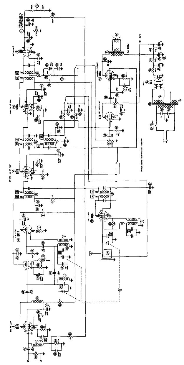
Figure 23. An AM-FM Broadcast Receiver.

Figure 24. The RF and IF Sections of the Popular Model 650 Receiver. These Circuits are Widely Copied.

The relative narrowness of the sound IF band pass and the fact that the response curves are usually symmetrical and peaked makes it possible to carry out the alignment using an RF signal generator and a VTVM. The signal generator would connect to the same points indicated for the sweep generator and the VTVM would go to the same places used by the oscilloscope. The generator would then be set to the sound IF frequency, say 21.00 mhz, and each of the IF coils would be peaked for maximum reading of the VTVM. The signal would be unmodulated.

Use of an RF signal generator and a VTVM for sound system alignment is n o t as desirable as the visual .method but it can be used and will provide satisfactory results. It is a simpler method and one which most servicemen find easier to perform. How ever, it presents a somewhat limited picture of circuit conditions which can sometimes be misleading. Once a serviceman becomes familiar with sweep signal alignment, he seldom returns to the RF generator VTVM method.

VIDEO IF SYSTEM ALIGNMENT

The use of sweep signals as a method of alignment reaches its greatest effectiveness in the video IF section of a television receiver. Not only is the response curve here not symmetrical ( except as noted later), but the bandpass is extremely wide (4 mhz) and for proper operation, specific frequencies should occupy certain selected positions on this curve. While an approximation of this curve can be obtained using an AM signal generator and a VTVM, optimum results can only be achieved by actually sweeping out the response curve and inspecting it visually by eye and electrically with a marker signal.

A video IF system that i s widely followed in conventional TV receivers is the circuit shown in Figure 24. The tuning circuits employed are all iron core single peaked coils, each resonant to a different frequency. Coupled to several of the coils are absorption traps whose purpose it is to prevent certain signals from reaching the video detector. In the case of L12, the energy thus absorbed is transferred to the sound system; in all other instances the energy is dissipated in the trap.

The manufacturer of this receiver recommends a two-fold approach to its alignment. Since all of the coils and traps peak to specific frequencies, it is suggested that each unit be adjusted to its peak frequency first, using an AM signal generator and a VTVM. Then, a sweep generator and oscilloscope would be brought in to develop the overall response curve and to permit such correcting adjustments to be made as would be necessary. This might seem like double work but when the circuits are grossly out of adjustment, or the procedure is unfamiliar, it i s really the quickest method. After we have examined the method, suggestions will be given which could help to shorten the time by proceeding directly with the sweep alignment.

To start as suggested, the AM signal generator is connected to test point 9 in the mixer grid circuit.

The VTVM is placed across the video second detector load resistor, R137. The power in the receiver and in the instruments are turned on and the units are permitted to warm up. The bias on the first three video IF stages in Figure 24 is set to -3 volts, this being the normal value encountered in operation . Then the signal generator is set to each of the following frequencies, in turn, and the indicated slug rotated for minimum reading on the VTVM. In each instance the generator should be carefully set to insure that it is exactly on the frequency desired.

21.25 mhz - L12 (In tuner)

21.25 mhz - T105 (Top slug)

27 .25 mhz - T103 (Top slug)

19. 75 mhz - T104 (Top slug)

Each of these coils is an absorption trap, designed to remove the energy of the frequency to which it is resonant. That is the reason for the minimum meter indication. This done, the generator is next set, in turn, to each of the frequencies given below and the specified slug rotated for maximum reading on the VTVM. (Bias value remains at -3 volts.) 21.8 mhz – L11 (In tuner)

25.3 mhz - T103 (Bottom slug)

22.3 mhz - T104 (Bottom slug)

25.2 mhz - L183 (Top of chassis)

23.4 mhz - L185 (Top of chassis)

These coils form the tuning circuits of the video IF system and hence they are set for maximum indication.

We are now ready to run a sweep test on the entire IF system. In place of the VTVM we would substitute an oscilloscope with the vertical input terminal connected to the junction of R137 and L188 through an isolating resistor of 10,000-ohms. The scope ground terminal goes to the receiver chassis.

It is also desirable to connect a capacitor between 100 and 1000 mmf across the oscilloscope input terminals in order to sharpen, the marker pips on the scope screen. Use the lowest value capacitor that gives the best results.

Injection of the sweep generator signal can be made at test point 9 (which, in the Standard Coil tuner is particularly easy to reach), or by direct connection to the mixer grid, or by attaching the signal lead to the mixer tube shield.* Be sure the tube shield is set away from the chassis. The sweep generator frequency for the circuit in Figure 24 would be set to approximately 23.5 mhz and adjusted to sweep over a 6 mhz range. The generator ground terminal attaches to the receiver chassis. Also the equipment should be set up, as outlined previously, for deflecting the oscilloscope tracing beam with a 60-cycle sine wave voltage. This voltage may be obtained either from the s we e p generator or from the oscilloscope, if the latter has a phasing control to use with it. Marker injection (after the response curve has been obtained) may be accomplished by any of the methods outlined previously in the discriminator discussion.

We are almost set to go, but one more preparatory step still remains: The setting of the bias on those stages which are controlled. In the circuit in Figure 24, the grid bias on the first three video IF stages are manually controlled by the picture ( contrast) control (R131). As this control is turned clockwise, the bias is reduced; as it is turned counter-clockwise, the bias is increased. It has been found that with a change in bias, the input impedance (here, notably the input capacitance) of a tube changes and this will alter the resonant frequency of the tuned circuit connected across the tube input. To derive the greatest benefit from an alignment, the grid bias of the con trolled tubes should be set to the value it will possess under operating conditions. With signals of moderate strength, this value is -3 volts# and the picture control would be set for this value. If the receiver employs a.g.c., then a fixed 3 volts (from a battery) should be inserted into the a.g.c. line with the negative end connecting to the line and the positive terminal to the chassis.

(In fringe areas or wherever weak signals are encountered, the recommended bias is between 1 and 1.5 volts. However, under these conditions, you might not align the response curve to the same shape as you would for normal signals. This will be considered presently in more detail.) A good precaution to observe before commencing the alignment is to disable the local oscillator in the receiver. This can frequently be done by pulling the oscillator tube out of its socket. If the oscillator and mixer tubes are in the same envelope, or if the filaments are series wired, tube removal is not feasible.

In this case it may help to unsolder one of the oscillator connections or perhaps rotate the tuner to a non-interfering position. In the Standard Coil tuner the oscillator can be disabled by carefully rotating the tuner turret or drum until it is balanced on one of the ridges between e a c h position where contact i s made with the tuner circuits. If this precaution is not taken, spurious responses set up by the oscillator voltage beating against the sweep generator signal can interfere with the response curve, either distorting it or else swamping it altogether.

Now, if every step has been carefully observed, then some sort of indication should be observed on the scope screen. If there is no indication at all, check the oscilloscope first to see whether it contains any visible trace at all and if it does, then check the set and sweep generator. (In line with suggestions made previously, the marker generator should not be connected until a response pattern has been obtained on the scope screen.) In the sweep generator, the following points should be examined:

1. Is the sweep generator putting out any signal at all? A fast way of determining this is to connect the sweep generator to the grid of one of the sound IF tubes in a receiver known to be in good condition. Set the generator frequency to the sound IF value (either 4.5 mhz in inter-carrier sets, or between 20 and 42 mhz in conventional sets) and turn up the volume control of the receiver. A 60-cycle rasping buzz indicative of the 60-cycle sweep ingrate in the generator will be heard. The sound will disappear as the generator frequency is altered.

*When the signal output of the generator is weak, it may be necessary to make direct connection to the mixer grid in order to obtain a usable indication on the VTVM. The other methods mentioned may not inject sufficient signal into the circuit.

While -3 volts is a value widely used, it is not the only one. Some manufacturers recommend higher voltages than this.

2. Is the instrument set to the proper range? To sweep over a range of frequencies from 21.5 mhz to 26.5 mhz, the tuning indicator should be at some point between these frequencies, preferably at the midpoint.

3. Is the output control set at maximum (to start)?

4. Is the sweep width control set at from 6 to 10 mhz?

In the absence of any response pattern on the scope screen, try rotating the sweep generator frequency dial from about 15 mhz to 30 mhz (assuming a video IF of 25 mhz or so). It is not uncommon to find that the dial calibration is off. When the error is small, it is of little consequence as long as the sweep generator is operating properly in all other respects.

The precise frequency of every point on the response curve is determined by accurate markers anyway.

Where the dial calibration of the sweep generator is considerably off and the serviceman would either like to recalibrate it or reset it (if there is provision for this), the following method is very useful.

Take the sweep generator and reduce the sweep width to zero, converting the instrument effectively into a simple RF generator. Then connect its output into the input terminals of the germanium detector network shown in Figure 40 of this section. Across ·the same two input terminals feed the signal from a carefully calibrated marker generator covering the same frequency range. The other end of this detector connects to the vertical input terminals of an oscilloscope. The frequency at every setting of the sweep generator dial can now be checked against the marker generator by zero beating both signals.

This calibration can be carried out in short order and will reveal, with an accuracy equal to that of the marker generator, how far the sweep genera tor's dial readings are off.

With the instruments and the receiver in operation, some type of curve will appear on the oscilloscope screen. In spite of all the warnings that have been given concerning feeding in of too much signal, or of disabling the oscillator, or of carefully bringing in the marker signal after a response curve has been obtained, certain errors will be made which will distort an otherwise normal response curve.

Given below are a group of typically distorted or in correct curves such as the serviceman is likely to encounter when he has committed some error in his preparation for the alignment. The analysis of each curve is designed to help the technician avoid making these mistakes or, at least, if a mistake is made, to realize what has caused it.

Figure 25A shows a typical desired response.

Specific frequency values are included to identify various points on the curves, such information being determined with a marker generator, one point at a time.

Figure 25. (A) Ideal Response Curve. (B) Bias at -2.5 Volts. (C) Bias at -2.0 Volts. (D) Bias at -1.5 Volts.

Figure 26. Curves Obtained by Tuning the Set to Various Channels.

Figure 27. (A) Marker Generator Connected Directly to Grid of the First Video IF Amplifier. Strong Signal Output. (B) Marker Generator Connected Same as "A" but With Weak Signal Output. (C) Marker Generator Coupled to Grid of First Video IF Amplifier Through 75,000 Ohm Isolating Resistor. Strong Signal Output.

Figures 25B, 25C,and 25D show the effect of too little bias on the stages to be aligned. The correct bias should be -3 volts. At -2.5 volts the curve is not appreciably affected although there is a definite change in the contour of the curve along the top. The overall amplitude of the curve has increased, including that of the two smaller side peaks. The greater amplitude, of course, is a direct consequence of the bias reduction. With -2 volts bias, the curve has become distorted due to a certain amount of overdriving or saturation in the video IF amplifiers. This condition becomes progressively worse as the bias is reduced still further, (as in Figure 25D) and now the artificial flattening of both the main curve and its secondary side peaks is quite pronounced.

The next set of related curves are Figures 26A, 26B, and 26C and they show what can happen when the set oscillator is permitted to function during the alignment operation. Each of these curves was obtained by tuning the set to a different channel. Within an y one channel, rotation o f the fine-tuning control will cause the pattern shape to change.

Some injurious effects which can be caused by the marker generator are shown in Figures 27A, 27B, and 27C. In Figure 27A the marker generator is connected directly to the grid of the first video IF amplifier and the output of this generator has been turned up high. Result is a complete swamping of the response curve.

In Figure 27B the marker generator is still connected to the grid of the first video IF amplifier but its signal output has been considerably reduced.

Now, some semblance of the video IF response curve can be seen, although the marker generator loading is still quite evident. The loading is due to the very low input impedance of the marker generator. hi this respect it is important to keep in mind that if the marker generator is connected into the circuit at a point which is closer to the video second detector than the sweep generator, the impedance the marker generator shunts across the circuit will have a direct effect on the sweep generator signal passing through the system.

On the other hand, if the marker generator is placed ahead of the sweep generator (nearer to, or in, the mixer stage), its impedance will have no effect on any response curve seen on the scope screen. This would happen, for example, if we connected the sweep generator to the grid of the first video IF amplifier tube and the marker generator to the mixer grid. Now, the only way the marker can affect the response curve is by injecting too strong a signal.

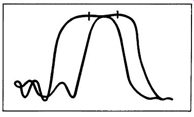
Figure 28. Sweep Generator Phasing Control not Properly Adjusted.

Figure 29. Insufficient Sweep Width for Phasing.

Figure 32. Improper Centering of Sweep Range (Too High).

In Figure 27C the marker generator is coupled to the grid of the first video IF amplifier through a 75,000-ohm resistor, thereby effectively isolating its low internal impedance from the video circuit. The big pip in the center of the response curve is now due to a strong output. If the marker generator output is reduced, the pip will attain its proper perspective and the response curve will be unaffected. All connecting leads should be kept as short as possible to minimize the effect of the inevitable shunting capacitance.

In Figure 28 the shape of the response curve is correct but due to an improperly adjusted phase control (on the sweep generator), two curves are seen.

The control should be adjusted until the two curves blend into one. In Figure 29 we have the same situation except that it is not possible to produce one curve at any setting of the phase control. Reason: The sweep width or sweeping range is too small. In crease the sweep width (to at least 6 mhz) and then a position on the phase control will be found where the curves will blend.

Incidentally, it should be noted that perfect blending is not always achievable. At some points the two curves will discernible. This can be disregarded, being due to an unbalance in the generator circuit.

As the sweeping range is increased, the area that the response curve occupies on the screen be comes progressively less. See Figure 30. A curve which is too narrow is difficult to work with. 6 to 8 mhz sweeping range for a 4 mhz bandpass is sufficient.

There is no need to go beyond this.

In some instruments, however, it is not unusual to find that a 6 to 8 mhz sweeping range is obtained only when the range indicator is turned to its extreme clockwise position.

When the sweep generator is being set up, its dial should be turned to the center frequency of the band being swept over. Thus, if the bandpass from 22 to 27 mhz is to be observed, the generator should be set at (or near) 24.5 mhz. If the center of sweep frequency is too low, Figure 31 will result. If the center of the sweep frequency is too high, Figure 32 will be obtained. Whenever both ends of a response curve are not at the base or lowest point on the ob served pattern, you can be sure that the full band is not being swept over.

A common error made by many servicemen results in the pattern shown in Figure 33. Everything has been properly connected here, except that the oscilloscope is still using its saw-tooth deflection voltage to sweep the beam across the face of the screen. To obtain the proper beam motion correctly synchronized to the sweep of the frequencies across the band, the internal sweep of the scope should be turned off and 60-cycle sweep voltage obtained from the generator itself.

The foregoing patterns are representative of those most frequently encountered by servicemen in their failure to obtain the proper response curve. If you study each one carefully and learn why it occurred, your chances of making the same error will be materially lessened.

*It is not uncommon to find a symmetrical response curve when the video IF system does not contain any trap circuits.

Figure 30. Curve Caused by too Great a Sweep Range.

Figure 31. Improper Centering of Sweep Range (Too Low).

Figure 33. Curve with Incorrect Scope Deflection.

Figure 34. Overall Video IF Response Curve Recommended by a Large Manufacturer for his Sets.

Figure 35. The Overall Video IF Response Curve Recommended by Another Manufacturer. Note Dip in Center of Curve.

The ideal video IF response curve is the one shown in Figure 25A. This curve has the proper slope on the video carrier side, has a full 4.0 mhz bandwidth, and decreases to the proper level at the trap frequencies. There are a number of sets on the market from which such response curves will be obtainable.

But the longer you work with television receivers, the more you come to find that there are also many sets from which you will not be able to obtain this shape curve. This one manufacturer shows the overall response curve of Figure 34 from mixer to video second detector. Note that the bandpass here is 3. 5 mhz ( which is not bad at all), and the curve is quite symmetrical.* Another manufacturer indicates in his service manual that the video IF response has a pronounced dip in the center of the curve. (See Figure 35). He recommends that this dip should not extend more than 30 per cent of the overall height of the curve. Other manufacturers state that the dip should not exceed 10 percent.

Here you have but a few of the variations that you will find among different sets when checking their IF response. For their particular circuits, under the policies of their design, these curves are "normal" and there is little the serviceman can do to change them--even if he should be so inclined. Try to strike the best compromise between amplification and bandwidth, emphasizing amplification in weak signal areas and bandwidth in strong signal areas.

As indicated on the video IF response curve, the placement of the video carrier and the trap frequencies are most important and should be carefully checked. This is done by setting the marker genera tor to each of the frequencies to be checked and noting where the pip falls on the response curve. Checking the video IF carrier and all other frequencies which fall fairly high on the response curve is readily carried out because no difficulty is encountered in seeing the marker pip. Within the trap hollows, how ever , the pip disappears and so you can never be completely sure whether the trap circuit is being aligned precisely on frequency.

One way to overcome this is to gradually reduce the sweeping range of the generator while the marker generator is kept at the frequency of the trap. Eventually, the marker pip will become visible in the trap and then the trap circuit can be adjusted for minimum height of the pip. The center frequency of the sweep generator may have to be readjusted as the sweep range is reduced in order to keep the marker pip and the trap it is in visible on the screen.

MODIFIED VIDEO IF ALIGNMENT

Most recommended procedures for aligning the video IF system specify first the individual peaking of the various video coils and traps, followed by an overall sweep alignment. Where it is desired to run a check on a receiver and there is no reason to believe that the system is grossly misaligned, it is often possible to omit the preliminary coil peaking steps and proceed directly with the sweep alignment.

In order to carry this out properly and in minimum time, the various slugs must never be haphazardly rotated. After the curve has been produced on the screen, use the marker generator to check its band width and the placement of the various key frequencies s u c h as the sound and video carriers. With this information, you are then in a position to make such corrections as are needed. For example, if you find that the video carrier is located too far up or down on the side of the response curve, then you would tune the slugs of those video IF coils whose resonant frequency was close to that of the video carrier. In the circuit of Figure 24, these would be T103 and L183 since their frequencies are, respectively, 25.3 mhz and 25.2 mhz and rotating their slugs would affect the side of the response curve containing the video carrier (frequency of 25. 75 mhz). Also effective here is the 27.25 mhz trap (in T103) and it, too, could be adjusted.

At the other end of the curve ( where the IF values are lower but which govern the higher picture frequencies), L11, T105, and T104 would have the greatest effect in altering the shape of the curve.

Finally, for the flat-top center portion of the curve, we would turn to L185 (23.4 mhz). Note that these adjustments are all interdependent to some extent and while their effect will be greatest on the section of the curve containing their frequencies, they will also influence, to some extent, all other portions.

This may require a certain amount of compromising between adjustments but if you proceed carefully, not too much difficulty will be encountered--certainly no where near as much as you would fall heir to if you turned slugs haphazardly. This modified procedure is not recommended for the beginner, but the experienced serviceman employs it frequently.

Often overlooked in alignment is the effect that the traps have in establishing the steepness of the sides. As you move the trap in toward the main body of the response curve, the side facing the trap tends to become steeper. If the slug is rotated too far, however, the trap will enter the response curve itself and tear a hole in it.

Figure 36. (A) Normal Video IF Response Curve. (B) Modified Response for Fringe Operation.

Figure 37. In an Intercarrier Receiver, The Sound Carrier Should Receive no More Than 5% of the Total Amplification Available in the Video IF System.

CURVE ALIGNMENT FOR FRINGE AREA OPERATION

Many television receivers are located in areas where the amount of signal available to the receiver is extremely small, possibly on the order of 50 microvolts or less. Under these conditions, it has been found desirable to modify the video IF response curve fr o m it s normal configuration t o the shape shown in Figure 36. The response to the higher video frequencies has been sacrificed in order to raise the amplification accorded the carrier and the adjacent low video frequencies. The sound carrier still receives its normal amount of amplification.

One precaution should be observed when making this modification. Manufacturers usually indicate that video alignments should be performed at a certain bias value. The figure generally given is -3 volts.

Under weak signal conditions, the bias will be considerably under this value, possibly less than -1 volt.

Since the set will operate with this type of signal, it is suggested that the bias value be determined with the set operating in the home and then aligned at the shop with this bias value.

The narrowing of the video IF response reduces the overall receiver bandwidth to approximately 2.5 mhz in place of the customary 3.5 to 4.0 mhz. Because of this it is not necessary that the video frequency amplifiers following the detector possess any wider response. Advantage can be taken of this to increase set gain by raising the value of the load resistors in the video detector and the following video frequency amplifiers.

An increase of 75 to 100 percent is recommended. Thus, if the load resistor value is 2200 ohms, a 100 percent increase will mean a resistor of 4400 ohms. Since resistors of this value are not common, any value close to it (as 3900 ohms or 4700 ohms) will do as well.

INTERCARRIER RECEIVERS

Intercarrier television receivers differ from the conventional receiver principally in the fact that the sound and video carriers remain together at least up to and frequently beyond the video second detector.

However, de spite the fact that the sound signal is permitted to reach the video second detector, it does so with very little amplitude and consequently it re-mains at approximately the same level on the response curve as it does in the conventional circuit. It may be moved slightly up on the curve, perhaps to a point where it receives about 5 per cent of the maximum amplification, but care should be taken to see that it goes no higher. See Figure 3 7.

The video IF system of a typical television intercarrier receiver is shown in Figure 38. There are three stages using four tuned circuits. Three of the circuits are bifilar coils, each containing closely wound primary and secondary windings tuned by a single movable slug. Two of the bifilar coils are resonant to 25.3 mhz while the third peaks at 23.1 mhz.

The recommended alignment procedure for the entire video IF system follows closely that outlined for conventional systems. First, each of the tuned circuits are peaked to their respective frequencies, with the AM signal generator connected either to test point D or to a loosely held mixer shield (that is not grounded). The VTVM indicator is connected across the video second detector load resistor or point A, whichever is mos t convenient. Since there are no traps in this system, each coil would be peaked for maximum meter indication.

After this has been done, a sweep generator replaces the AM generator and an oscilloscope is substituted in place of the VTVM. A 10,000-ohm isolating resistor is placed in series with the vertical input lead of the oscilloscope. After a response pattern has been produced on the scope screen, a marker signal is injected by one of the methods previously described. The various adjustments are then touched up as needed.

Figure 38. The RF and IF Stages of an Intercarrier Receiver.

In this circuit, as in the previous circuit, a negative 3 volt bias would be applied to the a.g.c. line, with the positive side of the battery attaching to the chassis. A lso, to prevent spurious responses, the oscillator should be disabled.

Throughout the alignment, particular attention should be given to the placement of the sound IF carrier. It must be positioned at least 95 percent of the way down the curve. It may be placed somewhat lower than this but it should not go any higher.

It is not the purpose of this section ( or this guide) to investigate each of the different types of video IF circuits that are in use but rather to note how test instruments can be employed to align such circuits.

In all instances it is recommended that the manufacturer's instructions be followed as closely as possible because while the general procedure outlined above will be sufficient in most instances, there appear, from time to time, certain variations that should be followed for best results. RCA, in their Mode 1 KHZS66 intercarrier receiver, stipulate that 330-ohm composition resistors be placed a cross certain portions of the video IF system. Emerson, in their Model 709A receiver, suggest that the response curve of the first or input IF transformer be checked separately by the use of a special detector network ( which we will discuss presently). The important thing is to know what you are looking for and how the equipment should be connected.

Figure 39. Representative Response Curves for Each of the Tuned Circuits (Except Traps) in Figure 24.

From time to time in your service or alignment work you will come across IF systems whose response cannot be brought in line with what is recommended or what it should be. The curve may be too narrow or you may find that while one section of the curve possesses the proper form, the other side does not.

Common causes of these conditions might be a defective tuning coil or slug, a shunting resistor which has radically increased or decreased in value, or even a defective tube. Whenever the tuning slug of a coil or transformer is varied, it should produce a very definite effect on the indicator (VTVM or oscilloscope). If it does not, check the coil and any shunting resistor.

If the shunting resistor has appreciably increased in value, it will narrow the response curve; if the resistor has decreased in value sufficiently, it will load down the coil to such an extent that slug rotation will have no effect. Utilization of this fact is made by RCA in many of their service manuals. They recognize that at times it may be desirable to observe an individual IF stage response pattern (perhaps when the proper overall response curve cannot be obtained). To do this, it is suggested that all other IF tuned circuits (except the trap circuits) be shunted with 330-ohm carbon resistors. The sweep generator would feed its output into the mixer tube (via its shield) while the oscilloscope would be connected across the video detector load resistor. With this set-up, the response pattern obtained will be essentially that of the un shunted stage. The effects of the various traps will also be visible. Representative response curves for each of the tuned circuits of Figure 24 are reproduced in Figure 39, together with that of the overall response curve. (These curves were obtained from the manufacturer's service manual

ALIGNING OTHER VIDEO IF SYSTEMS

Over 95 percent of the television receivers on the market can be aligned by the methods outlined above. About 5 percent of the sets employ trans former or complex coupling and for these circuits the manufacturer frequently recommends a stage-by stage alignment which differs in many respects from the foregoing procedure. The best way to illustrate this type of alignment is to follow through a step-by step adjustment of a representative circuit. In the material to follow, the circuitry from a Du Mont receiver is used.

The equipment required consists of a sweep generator, a marker generator, an oscilloscope and an RF probe. Everything but the probe has been employed before and the reason for the probe is quite simple. If you want to observe the signal at the plate of any IF amplifier, it first must be rectified or detected before it can be applied to the vertical input terminals of the oscilloscope. In all previously de scribed alignments the video second detector served to perform this function. However, when you wish to observe the response of a single IF stage, you must obtain the signal at the plate of the video IF stage ; you cannot wait until the signal has passed through the remaining IF stages and the second detector before applying it to the scope.

The additional probe indicated above serves to take the signal at any point in the video IF system, detect it, and apply the rectified voltage to the vertical input terminals of the scope.

Figure 40. A Probe Detector Recommended by DuMont for Use in Their Video Circuits. There are Many Variations of This Circuit.

Figure 41. Video IF System of a DuMont Model RA-105 Television Receiver.

Figure 40 shows the circuit of a probe detector recommended by the manufacturer. (There are many variations of this circuit, all functioning in the same manner.) Detection is accomplished with the 1N34.

When constructing this unit, make it as compact as possible in order that its input capacitance will have as little disturbing effect on the IF circuit as possible.

In using this detector, the output would be fed to the vertical input terminals of the oscilloscope. The in put terminal ( or probe end) would touch that point in the circuit where we wished to observe the signal.

The ground terminal would goto the receiver chassis.

The video IF alignment of the Du Mont video IF system (shown in Figure 41) would be carried in the sequence of steps given in Table 1. Wherever a response curve is to be obtained, an illustration of that curve is given. This enables you to compare what you obtain with an average curve recommended by the manufacturer.

The alignment table commences with the adjustment of the tuning circuits contained between the plate of the final video IF tube (V203) and the video second detector (V204). Since the oscilloscope is placed beyond the detector, no special probe is needed.

The next step is the setting of the a.g.c. bias to -3.2 volts for the first two video IF amps. The third video IF amplifier is not controlled and so it can be adjusted before the bias was set.

Steps 3 and 4 of Table 1 concern the adjustment of the sound trap (21.9 mhz) and the adjacent channel sound trap (27.9 mhz). Both are set, by means of an AM signal generator, for minimum output. To use the scope as an indicator, simply amplitude modulate the carrier with a 400-cycle audio note. After demodulation of the signal in the video second detector, the 400 cycle note would appear on the scope screen. The traps would be adjusted for minimum amplitude of the 400-cycle wave in each instance.

In step 5 the sweep and marker generators are moved to the grid of V292, the second video IF amplifier while the oscilloscope remains beyond the video detector. L207 and L208 are now adjusted to give the curve shown in Figure 42B. This curve represents the response of the video IF system from the grid of V202 to the video detector. In essence, then, it covers two video IF stages.

The first use of the special probe detector comes in step 6 where it is desired to view the response of the tuning network located between the plate of V201 and the grid of V202. The sweep and marker signal generators go to the grid of V201 while the probe touches the plate of V202. The probe output then connects to the oscilloscope. The recommended response pattern for the network between V201 and V202 is shown in Figure 42C. Any deviations that might be observed should be correctable by adjusting L204 and L206.

In step 7, an overall check is run on the video IF system from the grid of V201 to the video-detector.

This means that the sweep and marker signal generators remain at the grid of V201 while the scope is moved back beyond the video detector. The response curve for this section of the IF system is shown in Figure 420. In step 8 we return to the alignment and viewing of a single stage (between the plate of .,the mixer and the grid of V201) and again the probe detector is required. For the final step, the overall IF response is viewed.

The alignment of a complex coupled system is a rather lengthy procedure, as the foregoing description indicates. However, unless the effect of adjusting e a c h of the tuned circuits on the overall response is known, it would be a difficult matter--if not an impossible one--for someone to attempt an overall alignment rather than the stage-by-stage procedure given. There are too many interlocking adjustments to be made.

-----------

TELEVISION AND FM RECEIVER ALIGNMENTS

Table 1 A Video IF Alignment Chart for the Circuit Shown in Figure 41. (The Word Wobb Refers to a Wobbulator Which is Another Name for Sweep Generator.

Figure 42. The Response Characteristics of the Tuned Circuits in the IF System of Figure 41.

Figure 43. Circuit Diagram of the Standard Coil Tuner.

SWEEP ALIGNMENT OF THE RF STAGES

The front end section of a television receiver possesses a greater overall bandpass ( 6 mhz) than either the video or sound IF stages that follow it. To attain this bandpass, the tuning circuits are heavily loaded by a combination of shunting resistors and the relatively low input impedance of vacuum tubes at high frequencies. There are a number of front-end tuners in use of which the most popular is the Standard Coil tuner shown in Figure 43. This is a turret type of tuner containing separate removable RF and oscillator coils for each of the twelve VHF t e le vision channels. There are only three adjustments for the RF coils on all channels (C2, C3, and C4 in Figure 43) and these are set so that the most uniform response is obtained on all local channels. The oscillator coils have a tuning slug for each channel, this being required since the oscillator generates a single frequency per channel and it is relatively easy for this frequency to drift too far to one side or the other.

Alignment of the RF stages carries with it a number of precautions that must be observed if the job is to be properly carried out. First, there is the matter of matching the sweep signal generator to the receiver input terminals. Most sweep generators have an unbalanced output with impedances between 50 ohms and 100 ohms. On the other hand, television receivers possess either a 75-ohm unbalanced input or a 300-ohm balanced input. The 75-ohm unbalanced receiver input can usually be connected directly to a generator whose output is similarly unbalanced and whose impedance lies between 50 to 100 ohms without causing appreciable mismatching. However, when you attempt to connect such a sweep generator directly to the input terminals of a 300-ohm balanced receiver, the response pattern will be sufficiently affected to result in misadjustment of the circuit trimmers . (The input tuning circuits of a television receiver contribute to the shape of the overall RF response curve and when the proper matching is not employed between instrument and receiver, the tuning curve of this input circuit is affected. This, in turn, alters the overall pattern.) To match an unbalanced sweep generator to a 300-ohm balanced television receiver, an arrangement such as shown in Figure 44 would be employed. One series resistor has a fixed value of 150 ohms. The other series resistor has a value which depends upon the impedance of the sweep generator output; this is true also of the shunt resistor, Ro. The resistors should be of the non-inductive variety, preferably carbon or of composition construction. If the attenuation introduced by the resistors reduces the signal too much, a matching network using sections of a 150 ohm twin lead line may be formed. See Figure 45.

It is never good practice to align a strange tuner without having the manufacturer's alignment instructions on hand (unless this cannot be helped).

Figure 44. Resistive Network to Match Sweep Cable Impedance to Receiver Input.

Figure 45. How to Match an Unbalanced 75 Ohm Coaxial Cable to a Balanced 300 Ohm Impedance. Courtesy of Sylvania Electric.

Figure 46. RF Response Curve.

Some tuners, for example, must be removed from the receiver for the alignment. This is usually necessitated because only by removal can certain necessary adjustments be made. For other tuners, special jigs are required. Finally, the sequence in which the adjustments are made is frequently of great importance and this information, again, is available only from the manufacturer. Other factors which should be checked carefully in RF alignment is the value of bias re commended for the RF amplifier, whether or not the local receiver oscillator is to be cut-off, and whether the mixer plate tuning circuit is to be shorted out or otherwise modified to prevent it from affecting the RF response. RCA, in their Model KCS67-68 receiver, states that the tuner is to be aligned using zero a.g.c. bias and the output co-ax cable which connects the mixer plate to its tuned circuit is to be disconnected from this transformer and terminated by a 39-ohm resistor. Philco, in some models, uses -1.5 volts bias and shunts a 330-ohm resistor across the first IF coil to eliminate the absorption effect of this coil on the response curve. Pay particular attention to these pointers or you will not obtain the response curve indicated in the service manual.

Since the RF tuner in Figure 43 is used quite extensively, it may be instructive to examine its alignment procedure. The sweep generator is connected to the receiver input terminals through an appropriate matching network. The oscilloscope vertical input terminal connects to test point 9 through a 10,000-ohm resistor and the oscilloscope ground attaches to the receiver chassis.* The scope beam should be driven by a 60-cycle sine wave voltage obtained either from the sweep generator or from the oscilloscope if the latter contains a phase control.

The marker signal, when it is needed after a response curve has been obtained, would be loosely coupled to the sweep generator, either by connection through a small (5-10 mmfd) condenser, or by laying the marker generator output cable across the resistive matching network.

The negative terminal of a 1.5-volt battery is clipped onto the a.g.c. wire (D in Figure 43) and the positive terminal goes to the chassis. If it is found difficult to obtain a curve of sufficient amplitude, the battery can be removed and wire D simply grounded to the receiver chassis.

With the equipment in operation after an appropriate warm-up interval of 10 to 15 minutes, the receiver is tuned to channel 12. The response curve sought for this channel is shown in Figure 46. If the curve observed does not possess this form, adjust C2, C3, and C4. Adjusting C3 will generally shift the center of the response curve in relation to the video and sound carrier markers. C2 and C4 should be alternately adjusted for best gain with flat top appearance consistent with proper band width and correct marker location. Do not overly broaden the curves as this will result in a loss of sensitivity.

After the curve for channel 12 has been obtained, each of the other channels should be checked in turn.

In each instance, the marker generator frequency would be changed to the corresponding video carrier frequency and sound carrier frequency for the particular channel being tested. None of the RF coils possess individual adjustments and ordinarily the C2, C3, and C4 settings established for channel 12 will provide satisfactory response curves on all channels.

However, if reasonable alignment is not obtained on a particular channel, (a) check to see that coils have not been intermixed, or (b) try replacing the pair of coils for that particular channel, or (c) repeat the C2, C3, and C4 adjustments for the weak channel as a compromise adjustment to favor this particular channel. If a compromise adjustment is made, other channels operating in the locality should be checked to make certain that they have not been appreciably affected.

The foregoing outline represents the alignment procedure for one type of tuner and other units have other methods of approach. In a 11 RF alignments, follow the manufacturer's instructions closely.

*The mixer, being essentially a detector, provides the oscilloscope with a demodulated voltage, Should the response pattern of the RF amplifier stage itself be desired, then an RF probe would be required.

HF OSCILLATOR ADJUSTMENT

In every television receiver, the high frequency oscillator o p e r at e s, on any given channel, at one particular frequency. If the oscillator frequency should drift, the sound and video IF frequencies which are produced by beating the HF oscillator against the incoming signal will also change. With sufficient drifting, the set maybe detuned to an extent which will produce a fuzzy picture and distorted ( or no) sound.

To provide the viewer with some means of overcoming oscillator drift, nearly all television receivers possess a fine tuning control. When aligning the oscillator on each of the channels, this control is set (and left) at mid-position. This is done to insure that sufficient correction is available to the viewer should the oscillator drift in either direction.

There are a number of methods by which the oscillator can be accurately set on frequency for the channel or channels on which the set is used. Probably the simplest method, the one most widely practiced by servicemen, and, in a sense, the most accurate method, is the alignment of the oscillator using a received television signal. The set is left in the cabinet, but the dial plate ( or whatever other obstruction is in the way) is removed in order that the oscillator tuning slug may be reached. The antenna is connected to the receiver and a local station is tuned in. The fine tuning control is set to mid-position. Then the alignment screwdriver (non-metallic, preferably) is inserted into the oscillator slug and the slug position adjusted for best picture and/or loudest sound depending upon the receiver. In Intercarrier sets, the slug adjustment is made with an eye on the picture rather than the sound because it will normally be found that where the sound is loudest does not necessarily represent the optimum operating point so far as the picture is concerned.

On the other hand, in conventionally operated receivers, the oscillator slug is adjusted for loudest sound and, if the set is operating normally, the picture will be best here, too. It is important that this difference between systems be kept in mind.

With the TV signal method, the set is adjusted on each channel where a signal can be received. The unused channels are disregarded.

A second method of alignment can be employed in those receivers where the correct HF oscillator frequency for each channel is known. This information may be obtained directly from the manufacturer's service notes or the serviceman can compute the proper value by adding the video IF carrier frequency to the channel's video RF carrier frequency. Thus, for channel 2, the video carrier RF value is 55.25 mhz and the video IF value is 25. 75 mhz. Added together, we obtain the oscillator frequency of 81.00 mhz. This procedure can be followed on all low band channels ( 2-6) because all TV receivers have the HF oscillator working above the signal frequency in this portion of the TV spectrum.

For channels 7-13, the HF oscillator usually is placed above the incoming signal, but it need not be and some manufacturers place it below the signal frequency. Where the oscillator frequency is below, we would subtract the video IF value from the video RF figure, rather than add the two.

Once the oscillator frequency for each channel is known, we would proceed as follows: A carefully calibrated AM signal generator is connected to the input terminals of the receiver (matching network not required) and set to the oscillator frequency for the channel to which the set is tuned. Let us say this is 81 mhz for channel 2. A wire is then connected from the mixer, point 9 in Figure 43, to grid of the first audio amplifier. The FM detector tube is removed to prevent any other signal from reaching the audio system. The oscillator fine tuning control is set to mid-position and then the tuning slug of the oscillator coil is carefully adjusted until a zero beat whistle is heard in the receiver speaker. This indicates that the oscillator signal beats with the generator signal in the mixer and the resultant difference frequency is transferred to the audio system where it can be heard. At zero beat, both frequencies are equal. If desired, an oscilloscope could be connected to point 9 and the zero beat observed visually.

A third method of oscillator adjustment is to set the AM signal generator to the sound RF frequency itself (59.75 mhz for channel 2, for example) rather than to the HF oscillator frequency as in the previous method. A zero center VTVM is then connected to the FM detector; for the ratio detector, it would be point A (and ground), Figure 2 and for a Foster-Seeley discriminator, it would be point A ( and ground), Figure .i. Then, with the set and equipment in operation, the oscillator slug would be adjusted for zero reading on the VTVM. Slight rotation of the slug in one direction will produce a negative reading; slight rotation in the opposite direction will produce a positive reading.

Be careful that the oscillator slug is not rotated too far in any one direction because it is possible to obtain a false zero reading. In the correct position, the action just described will occur. In a false zero position, you will not be able to go from one polarity w the other, with zero in between.

A fourth method of oscillator alignment which is sometimes recommended by manufacturers consists in connecting a sweep generator to the input terminals of the receiver through an appropriate matching net work. The output of a marker generator is then loosely coupled to the matching network as previously described . An oscilloscope is connected through a 10,000-ohm isolating resistor to the video second detector load resistor. Bias for the a.g.c. network would be set at -3 volts unless otherwise recommended by the manufacturer.

Figure 47. Overall RF and IF Response Curve of a Television Receiver Such as the One Shown in Figure.

Figure 48. A One-Stage Video Amplifier System.

With the set and test equipment in operation, an overall RF and IF response curve, such as shown in Figure 47, should be obtained. Note that this response c11rve is actually the same as the response curve of the video IF system alone. Now, with a non-metallic screwdriver, adjust the oscillator slug ( of the channel to which the receiver is tuned) until the sound marker pip falls into the hollow provided for it, as shown in Figure 47. In order to see the marker clearly, it may be necessary to advance the vertical gain control on the oscilloscope in order to blow up the sound trap portion of the response curve.

After the sound marker has been properly positioned, change the marker generator frequency to the video RF carrier value for that channel and note whether the marker pip appears on the response curve in its proper place. (This is also indicated in Figure 47.) A similar procedure can be followed for each channel. In each instance the sweep generator frequency and marker signal frequencies would be changed to suit the channel.

A similar procedure using the output of the FM detector (i.e., an S-curve) instead of the video IF system could be followed. The sound marker pip now would appear at the zero or center point of the S curve when the oscillator frequency is properly set. The reader will recognize that we are now doing visually exactly what was done previously using an AM generator and a VTVM. Aside fr o m alignment of the oscillator, this last method reveals that whenever an overall response test is run, the shape of the curve seen on the screen will be that of the last system through which the signal has passed. If the scope is placed at the video second detector (with the sweep generator at the receiver input terminals), then the curve viewed on the scope screen will be that of the video IF system. If the scope is placed at the sound FM detector, then an S curve will be seen.

In employing this fourth method care must be taken to see that the sound and video IF systems are correctly aligned before any oscillator adjustments are made. Also see that the oscillator tube shield plus all tuner shields are in place. Because of the high frequencies dealt with, any slight circuit disturbance, in the form of stray capacity or inductance, will alter the oscillator frequency. Another item of importance is the dial calibration of the marker generator. This must be accurate, otherwise the oscillator will be set incorrectly.

*There are some reservations to this statement which do not apply to normally operating TV receivers.

RESPONSE CHECKING OF VIDEO AMPLIFIERS

Most servicemen know that the tuned circuits in the RF and IF stages of a television receiver lend themselves readily to sweep signal alignment. Not so well known is the fact that the overall response of the video amplifiers can also be developed on a scope screen. The video amplifiers ( as distinguished from the video IF amplifiers) are those stages which follow the video second detector. There may be one stage, as in Figure 48, or two, as in Figure 49. There is never less than one and, in commercial sets, seldom more than two. The response of this stage (or stages) ordinarily extends from 30 cycles up to 3 or 4 mhz.

The low frequency response is upheld by special compensating networks, such as of C4B and R 51 in Figure 49. The extent of the high-frequency response is determined by the values of the load resistors (R50 and R55 of Figure 49) and the series and shunt peaking coils. Should any of these components change value or otherwise become defective, the effect on the response would make itself evident in the quality of the pictures produced on the screen.

The entire video signal must pass through the video amplifier stages before it reaches the picture tube and quality degradation in this section of the receiver is just as effective as poor alignment in any of the IF or RF stages.

The wide bandpass of the video amplifiers preludes point-to-point frequency checking just as it did in the IF and RF stages. To perform a sweep alignment, using .equipment that might ordinarily be found in the average TV service shop, we would take an IF sweep generator and connect its output across the input to the video second detector. This is shown in Figure 50. A 220-ohm resistor would have to be shunted across L16 in order that all frequencies produced by the sweep generator affect the video detector uniformly. T he sweep generator would be set to swing over the IF frequency range of this receiver (21.25 to 25. 75 mhz, here).

Figure 49. A Two-Stage Video Amplifier System.

Figure 50. How the Equipment is Set Up to Obtain Video Amplifier Response Curve.

Figure 51. An Ideal 4 mhz Video Amplifier Response Pattern.

The next step would be to connect a marker signal generator to the same point as the sweep generator, possibly through a 100 mmf capacitor. The marker generator would be set at exactly the video IF carrier value, in this instance 25.75 mhz. Now, with both these signals feeding into the detector, here is what happens. When the sweep generator is at 25. 75 mhz, the zero beat between it and the marker genera tor produces no output (actually only a DC voltage). As the sweep generator frequency swings away from 25. 75 mhz, the beating with the marker signal continues and so difference (and sum) frequencies will continue to be generated in the video detector. At 24. 75 mhz, the difference frequency is 1 mhz; at 23. 75 mhz, it is 2 mhz, etc. With an overall 5 mhz sweep (say from 20.75 mhz to 25.75 mhz), a continuously sweeping difference frequency signal from 0 to 5 mhz would appear at the output of the video detector and proceed through the video amplifier stages. At the picture tube some of these frequencies would be stronger than others be cause they received more amplification. If we now take a crystal detector and rectify this amplitude varying ( or modulated) signal and feed the amplitude variations to an oscilloscope, we will" develop the response characteristic of the video system between 0 and 5 mhz.

In order not to shunt too much capacitance across the output of the video amplifier system, the lead to the picture tube would be removed. Also, the scanning beam in the oscilloscope would be driven by the 60-cycle sine wave voltage obtained from the sweep generator. (If the oscilloscope has its own provision for supplying this voltage , this may be used instead.) With the equipment set up and operating, and the phase control properly set for a single trace, you may possibly obtain a pattern such as shown in Figure 51.

The zero beat point (representing zero frequency) is indicated by the marker pip hash. This pip may be in the center of the pattern or off to one side. When it is in the center, it signifies that the frequency in the sweep generator is swinging above and below the marker frequency which, for our present illustration is 25. 75 mhz. To move the zero beat indication over to the left, lower the sweep generator frequency. If this is done carefully and the sweep width is set to cover a range of 5 mhz, the zero frequency marker pip will be stationed at the extreme left-hand side of the screen and the shape of the pattern from this point to the right will represent the response characteristic of the video amplifier from 0 to 5 mhz.

Just what type of curve will be obtained will depend upon how well the video system was designed.

In very few instances will it look like the curve shown in Figure 51, which is an ideal curve and employed here mainly for comparative and instructional purposes. More likely the curve you obtain will look like one of those shown in Figure 52. These were taken from various commercial receivers.

Figure 52. The Video Amplifier Response Patterns of Several Commercial Receivers.

Once the curve is obtained, your next step is to check it at various points in order to determine at what frequencies the curve rises and where it starts to fall off. For this a variable marker pip is required and such a pip can be obtained from any AM signal generator operating between 500 khz and 5 mhz. Couple the output of this generator very lightly into the video amplifier circuit (by one of the methods outlined previously) so that the response curve is not disturbed.

Then by changing the frequency of the marker pip we can inspect the entire response curve, noting at ;hat point it rises and where it dips.

By means of the video amplifier response curve the serviceman can study the effect that various components have on it. Thus, for example, by increasing the plate load resistor (R50 and R55 in Figure 49), the curves amplitude will be found to increase but at the same time, the frequency bandpass will become narrower. A sharp rise in the curve near the high frequency end can frequently be traced to an open resistor shunting one of the peaking coils. Removal of the low frequency compensating networks will adversely affect the low frequency response, etc. A serviceman can gain a liberal education in television receiver operation by systematically changing the value of different components in a system and noting the effect on the response curve. While this may be somewhat beyond the province of everyday service work, it will provide the technician with a deeper and clearer insight into receiver circuit behavior and this knowledge can be of great value in television receiver servicing, especially when the cause of a certain defect appears obscure.